θ Car: Chandra AO11 proposal planning
updated: 15 March 2009
The RGS data
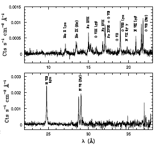
This fluxed spectrum was published in Naze & Rauw, 2008, A&A, 490, 801. The lines are unresolved with an upper limit of ~350 km/s. And although the f/i ratios were analyzed for N, O, and Ne, the constraints (r < 5 Rstar) are not very interesting.
With a long (125 ks) Chandra HETGS observation, we can address these two remaining open questions about the X-ray spectrum: (1) What are the widths of the emission lines? And (2) What constraints on the location of the hot plasma can be provided by the f/i ratio in Mg XI?
Note: We've reduced the exposure time from our original simulations (that had 200 ks). The other change in the global spectral simulations is the inclusion of non-solar abundances for N (enhanced by 3), C (reduced to 0.1), and O (reduced to 0.25). These values are taken from the introduction of Yael's 2008 paper, which references Hubrig 2008, and are also consistent with what Yael derives from the RGS data, reported on later in that paper.
Simulated data
I have simulated a 125 ks ACIS-S/HETGS spectrum (first order, both MEG and HEG) using the 2-T thermal spectral model fits reported in Naze & Rauw. These have:
solar abundances, except for C (0.1 solar), N (3 solar), O (0.25 solar)
kT1 = 0.16 keV
norm1 = 0.0007
kT2 = 0.39 keV
norm2 = 0.0016
NH(ISM) = 1.8e20 cm-2
There are a range of possible temperatures and abundances discussed in Naze & Rauw 2008. The ones we use here are representative. I used (vapec+vapec)*wabs in xspec, and fakeit, to make the models shown below.
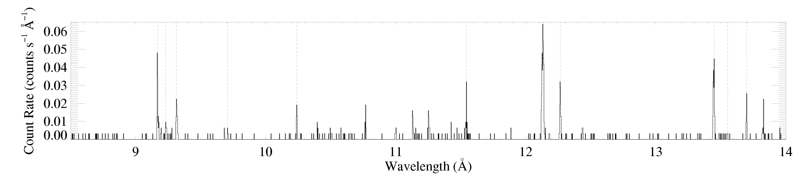
Below are the full MEG spectrum, a zoomed in view of the shorter wavelength portion of the spectrum, and the HEG spectrum (with the same zoomed in view). Note different y-axis range for each plot.
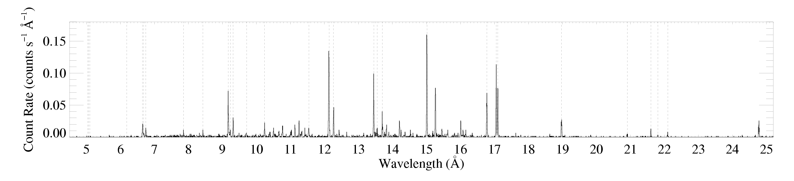
MEG

MEG
HEG
Note that there's no intrinsic line broadening in these simulations. And that the f/i ratios are all in the 'low density limit.' The total number of counts in these simulated spectra are 613 and 4174 in the HEG and MEG, respectively, coadded first orders.
Co-Is: should we multiply these models by the exposure time so the y-axes are in counts per A?
Fits to the simulated data
I'm putting off re-fitting the 2-T vapec model to look at constraints on parameters because... it's a stilted exercise and the results will be relatively meaningless. Co-Is: let me know if you disagree and think it's something we should discuss in the proposal. I could see putting one or even two sentences in about it. I mean, a secondary goal of our project is going to be to put better constraints on the temperature and abundance distributions in the emitting plasma (using the proposed HETGS data along with archival RGS data). But I think we can state that, without running reams of simulations for the proposal.
The two main goals of the proposal are (1) to constrain the widths of strong lines to see just how inconsistent with the expectations of the wind shock paradigm the data are and (2) to constrain the f/i ratio on Mg XI to put interesting constraints on the location of the X-ray emitting plasma.
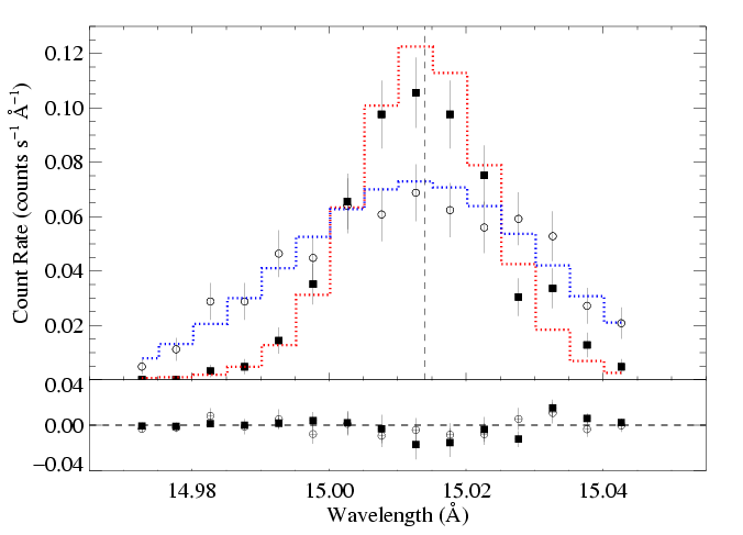
For the strongest line in the spectrum, Fe XVII at 15.01 A, we have 436 MEG counts (and 143 HEG counts). I re-simulated this line using the wgauss + pow model, twice: once with a line width (Gaussian σ) of 100 km/s, and once with 300 km/s. I then refit the simulated line profiles with a same type of Gaussian profile model (allowing the centroid shift and normalization, in addition to the line width, to be free parameters). Here are the two simulated datasets (100 km/s shown as filled squares; 300 km/s shown as open circles), along with the best-fit models in each case:
MEG |
[14.97:15.05]
powerlaw continuum, n = 2; norm = 1.97e-4 model with 300 km/s width: σλ = 337 +/- (316:353) km/s and 95% (300:375) model with 100 km/s width: σλ = 108 +/- (98:118) km/s and 95% (87:128) λo = 15.014 A |
So, we can recover intrinsic widths of 300 km/s and even 100 km/s with a high degree of accuracy, and we can easily tell these two widths - both of which are consistent with the unresolved lines in the RGS data - apart at >>95% confidence.
I will repeat this exercise for, say, the fifth strongest line in the spectrum, to show that we can do this analysis for a significant number of lines.
Here is a table that Yael put together, showing the B stars with X-ray line width determinations. I think delta Ori and sigma Ori AB are late O stars that are also relevant.
New: Simulations of the Mg XI complex for a 125 ks observation
I used hegauss + pow with normalizations based on the 2-T apec simulation. I made three different models and simulated 100 ks exposures for each grating using fakeit. These are shown below for the three cases R = 0.1, R = 0.6, R = 1.2, along with the best-fit models I obtained from fitting these fake datasets with the same type of hegauss + pow models. These models had five free parameters: R, G, σλ, δλ, and the normalization. Note especially the re-fit values of R and, even more importantly, the confidence limits on R. All the other four free parameters were allowed to vary while these confidence limits were determined. Detail is in the xspec log file.
Note that we show only the MEG here, but we simulated and fit the HEG too. Also, we don't list confidence limits on sigma, delta, and norm for simplicity, but they all varied in the fits and we calculated confidence limits on norm.
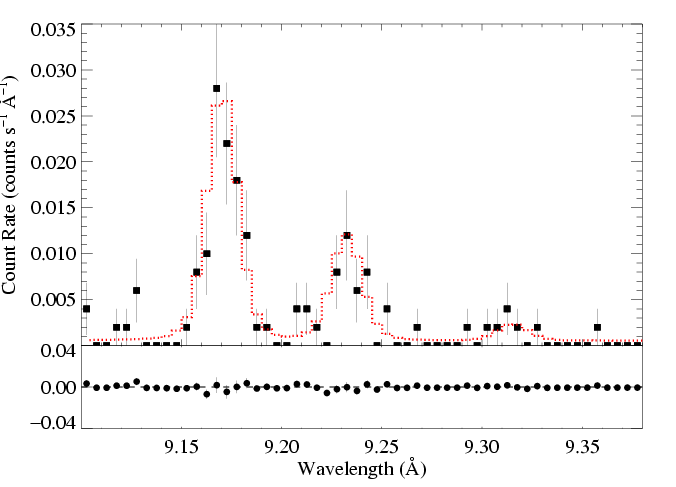
MEG: R = 0.1 simulation |
[9.1:9.4 Angstroms]
powerlaw continuum, n = 2; norm = 7.e-5 R = 0.16 +/- (0.08:0.27) (90% given by 0.04:0.36) G = 0.50 +/- (0.40:0.62) σλ = 75 km/s δλ = 46 km/s norm = 8.21e-6 C = 164.40 (N = 356) |
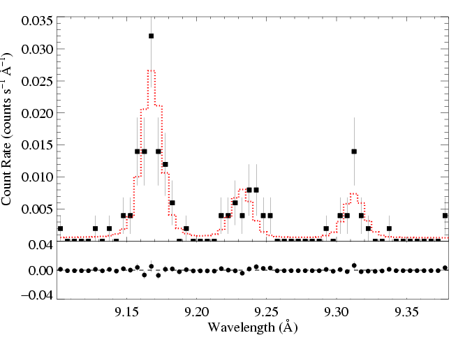
MEG: R = 0.6 simulation |
[9.1:9.4 Angstroms]
powerlaw continuum, n = 2; norm = 7.e-5 R = 0.81 +/- (0.56:1.16) (90% given by 0.44:1.46) G = 0.60 +/- (0.48:0.75) σλ = 26 km/s δλ = -5 km/s norm = 7.90e-6 C = 151.67 (N = 356) |
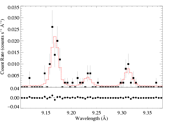
MEG: R = 1.2 simulation |
[9.1:9.4 Angstroms]
powerlaw continuum, n = 2; norm = 7.e-5 R = 1.39 +/- (0.81:2.10) (90% given by 0.58:2.82) G = 0.61 +/- (0.48:0.82) σλ = 22 km/s δλ = -27 km/s norm = 6.45e-6 C = 151.62 (N = 356) |
I plot the constraints on the formation radius, Rfir based on the fits to the simulated datasets with R = 0.1 and 0.6, below.
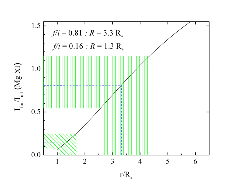
The model is from Blumenthal, Drake, and Tucker 1972, with the far-UV flux of theta Car scaled down by 20% from the beta Cru value. The take-home message from this figure is that we can tell f/i = 0.1 from f/i = 0.6, and thus can tell plasma just a few tenths of a stellar radius from the photosphere apart from plasma at 3 Rstar.
Putting the Mg XI f/i ratio in context: Here is the relevant figure from my 2008 paper on beta Cru:
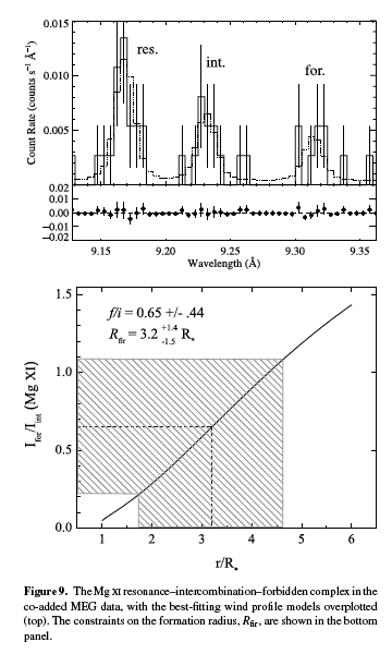
beta Cru (B0.5 III) has a photospheric flux very similar to theta Car's (B0.2 V).
Maybe we should emphasize the relationship to beta Cru in the proposal. Testing to see if there's another early B star with mysterious soft X-rays: large filling factor, narrow but resolved lines, f/i ratio indicates plasma well above the photosphere. We can emphasize this mystery in beta Cru (slow moving hot plasma far from the photosphere) and argue that the RGS data already suggest that theta Car is in the same category, and that Chandra will be able to say for sure. New: Yael suggested that we could hurt ourselves by emphasizing the "mysterious" nature of beta Cru.
last modified: 15 March 2009