|
|
(7/8/04) |
For those interested, all of the figures shown here as well as all of the workspaces, I/O files, and other miscellaneous items used to create them are available on my research webpage.
With the ultimate goal of modeling the neon gas cell experiments on the Z machine carried out by Jim Bailey (Bailey et al. 2001) and investigating different experimental setups for future gas cell experiments, David and I have been using the viewfactor code VisRad, 1-D Lagrangian code Helios, and the spectral synthesis code Spect3D, to respectively simulate the incident radiation field, calculate the time-dependent temperature and density distributions, and synthesize time-dependent absorption spectra for the old neon gas cell experiments. Before proceeding with simulations for future experiments with different setups, David and I would like to share with you what we have come up with thus far for the neon experiments and make certain that our simulations and results are reasonable.
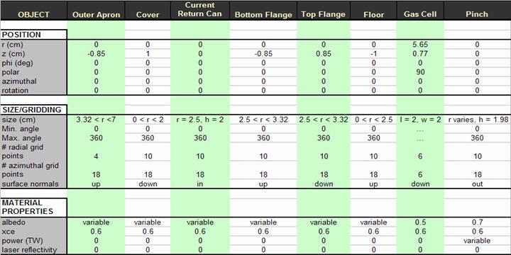
I created a workspace in VisRad using objects and associated parameters shown in the table below.
Click here or on the above image to download a Microsoft Excel Spreadsheet including the VisRad simulation parameters.
Click here to download the VisRad workspace for the 2-D gas cell.
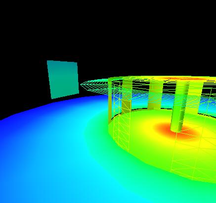
For this simulation, I used a planar gas cell with dimension 2 cm x 2 cm. It was located at a radial (parallel to the floor) distance of 5.65 cm and a z (perpendicular to the floor) distance of 0.77 cm. See below for a screenshot of the workspace.
|
In this image, the gas cell is visible to the left while the pinch and current return can are visible to the right. |
The current configuration of the holes, or slots, in the current return can provides an unobstructed view of the pinch from different horizontal positions provided that the gas cell is centered on a slot of the current return can. Certainly, one can imagine a different configuration in which the gas cell is not centered on one of the slots in the current return can, and thereby having some fraction (if not all of the pinch) blocked at some horizontal position(s) along the face of the cell. Previous simulations by Joe MacFarlane have shown horizontal gradients on the cell, so the apparent lack of horizontal gradients in our simulations has caught our attention and has given us cause to confirm that our configuration is correct. After reviewing screenshots from Joe Macfarlane's old simulations, we believe that he may have assumed narrower slots in the current return can. Thus, even if we have the azimuthal angle correct, our results could be incorrect if our slots are not of the right size.
Q1: What are the dimensions and geometry of the current return can?
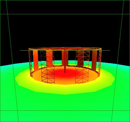
Although there is a complete lack of horizontal gradients along the face of the cell in our simulations, there is, however, variation along the vertical axis of the gas cell. The reason for this is that in our configuration a smaller fraction of the pinch is visible from the top of the gas cell than is visible from the center or bottom of the gas cell. See the images below for screenshots from the simulation workspace showing the view of the pinch from different locations on the gas cell and a schematic of the front of the gas cell with the viewing location highlighted.
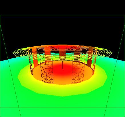
View of the pinch from the top of the gas cell. 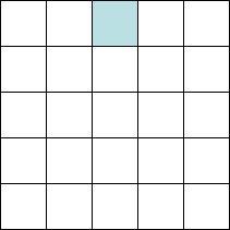
"TOP" |
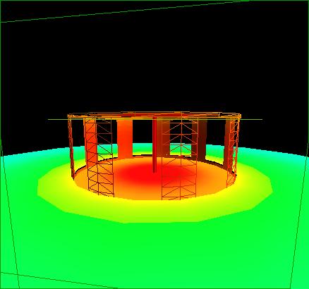
View of the pinch from the center of the gas cell. 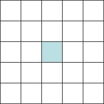
"CENTER" |
View of the pinch from the side of the gas cell. 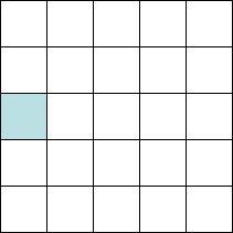
"SIDE" |
Notice how in the "top" viewing position, part of the pinch is blocked from view by the top flange on the current return can. From the "center" and "side" viewing positions, all of the pinch is visible, but a slight variation in the size of the slots or the azimuthal angle of the centroid of the gas cell could easily obstruct the view of the pinch from the "side" viewing position.
Using screenshots of the simulation for different times, I constructed a movie of the emmitted flux and emission temperature of the pinch and the incident flux on and the radiation temperature of the gas cell. Click here to see the movie. Two images of the gas cell are in the middle column of the animation; the top shows radiation temperature and the bottom shows incident flux. (Note: In future versions of the animation, we will be modifying the quantities and the views we show.) At later times in the simulation, the animation clearly shows a vertical gradient on the gas cell.
Q2: What is the shape, dimension, and location of the gas cell? What is the composition (and therefore albedo) of the gas cell surfaces? Is there a photograph of the cell?
As you can see in the table above, most of the objects in the workspace have a variable albedo. For each of these surfaces I used the same albedo model, a model which I obtained from Greg Rochau's old workspace. A plot of the albedo as a function of time is shown below.
Albedo Model |
Click on the image or here for a zoomed in view of the plot. Click here for a table of the albedo values as a function of time. |
Q3: Is this a good albedo model for the metal surfaces in the simulation? Should we be using different albedo models for different surfaces (e.g. are the floor, current return can, etc. gold? steel?)? If so, what albedos are appropriate for each?
I also obtained data for the time-dependent power and radius of the pinch from Greg Rochau's old workspace. The data is displayed in the following plots. Click on either plot for a zoomed in view.
Pinch Power vs. Time |
Pinch Radius vs. Time |
Using the data from the above plots and a few parameters of the pinch, I was able to calculate the time-dependent emission temperature of the pinch. See the plot below for the results.
Pinch Emission Temperature vs. Time |
Q4: Is our data for the time dependent pinch power, radius, and emission temperature reasonable? Do you have better data that we should be using? Also, is the data specific to shot Z543 reported on in Bailey et al. 2001? For new shots we might perform in the next year, do we expect significantly different pinch properties?
To investigate the spatial variation of the radiation field incident upon the gas cell, we used VisRad to output the incident spectrum on and radiation temperature of the three representative locations of the gas cell shown above in the figures comparing the different views of the pinch from the gas cell. See the two plots below for the visualization of these comparisions.
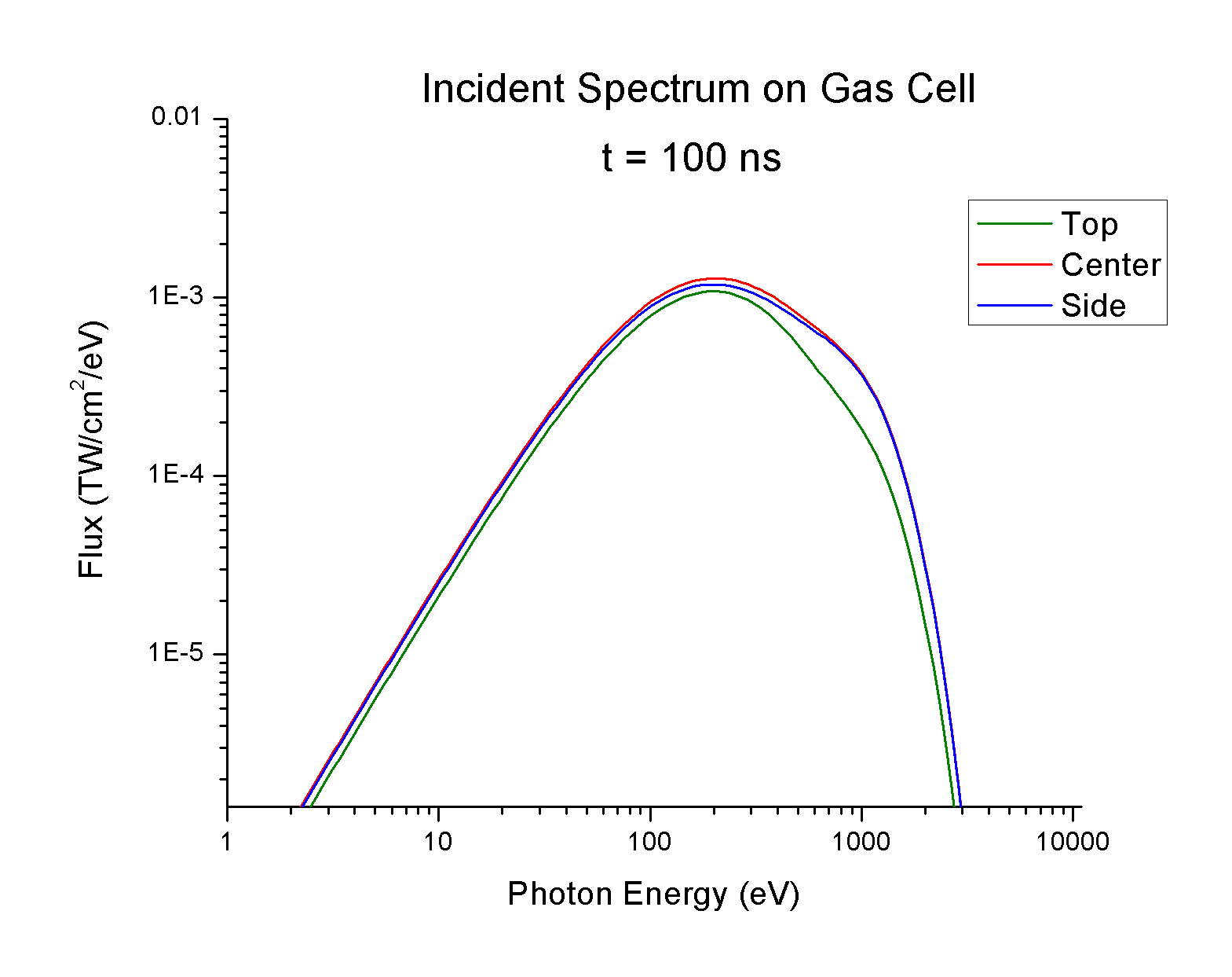
Spatial Variation of Incident Spectrum on Gas Cell |
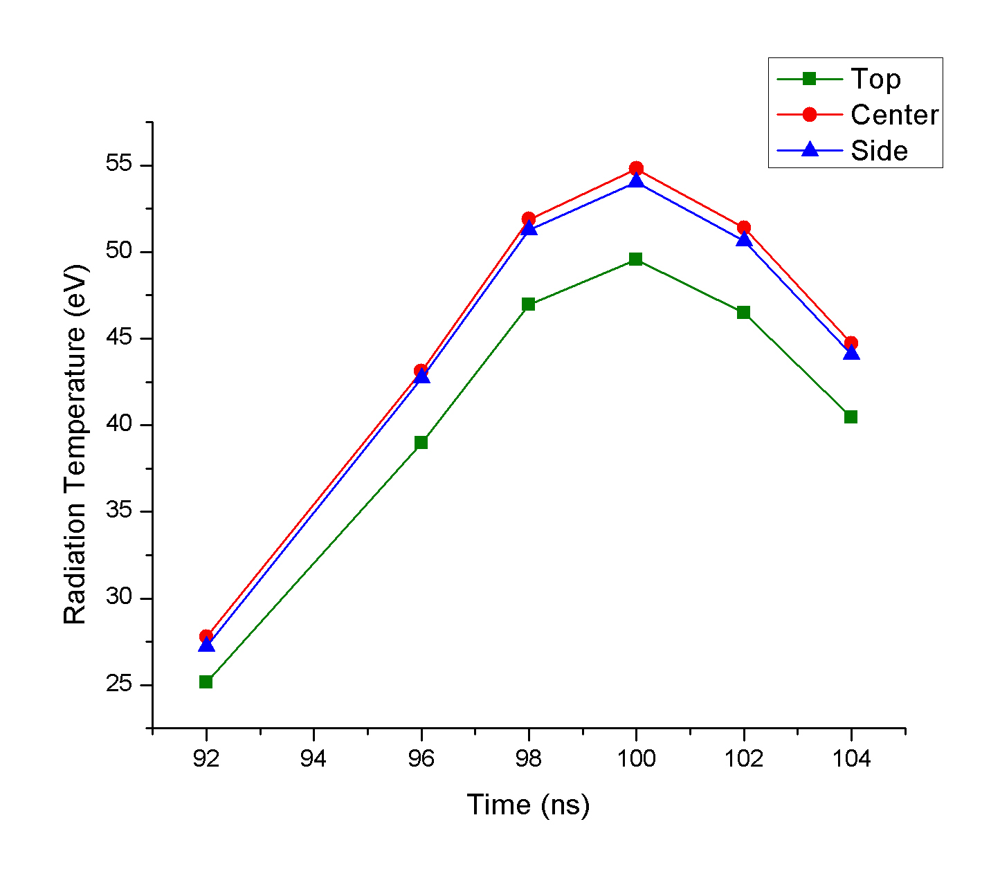
Spatial Variation of Radiation Temperature of Gas Cell |
These plots confirm our earlier observation from the animation that the top of the gas cell receives less flux from the pinch than does the rest of the gas cell. Further, the incident spectrum plot shows that most of the missing radiation at the top of the gas cell at t = 100 ns (peak of the pinch emission) is composed of higher energy photons (direct contribution from the pinch). The radiation temperature plot shows that the top of the gas cell consistently receives less flux throughout the experiment, and that the difference between the radiation temperature of the top of the gas cell and other areas of the gas cell is of similar magnitude at later times during the simulation.
In addition to investigating the spatial variation of the incident radiation field on the gas cell, we also looked closely at the field incident at the center of the gas cell, which we approximate as representative for the entire gas cell. First, we were interested in what contributed to the incident flux at the gas cell, so we plotted independently the spectra incident on the gas cell from different surfaces in the workspace.
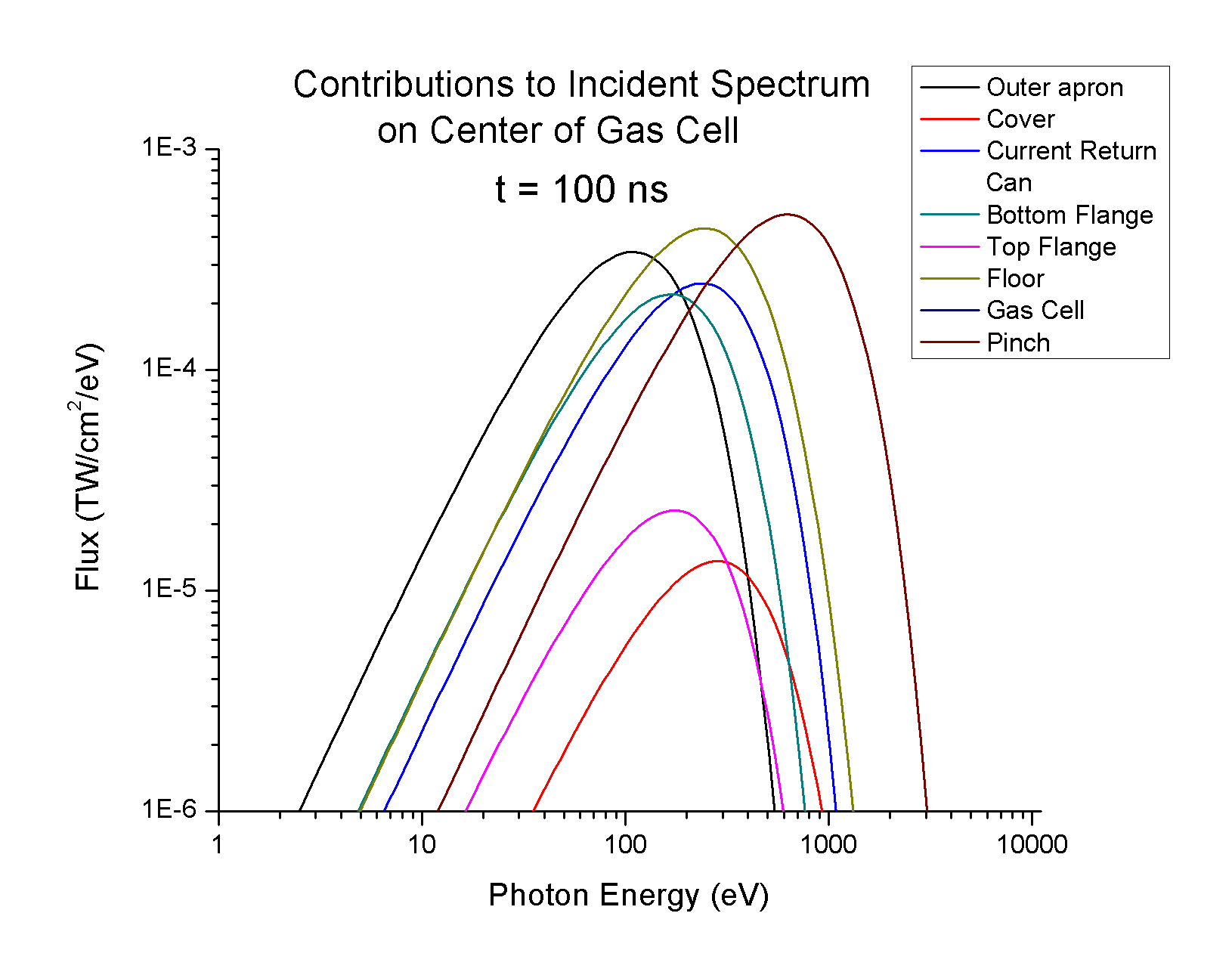
Incident Flux on the Center of the Gas Cell from Other Surfaces |
Not suprisingly, the pinch contributes the bulk of the high energy flux incident on the center of the gas cell at 100 ns, but it also interesting to note that the contributions of the other surfaces, especially for lower energies, is not negligible. This nonnegligible contribution from surfaces other than the pinch is precisely the reason why we are concerned about getting the time-dependent albedos correct for all of the surfaces in the simulation.
We also wanted to investigate how the incident spectrum on the center of the gas cell changed with time, so we used VisRad to output the incident spectrum at several times during the simulation, and used that output to produce the following plot.
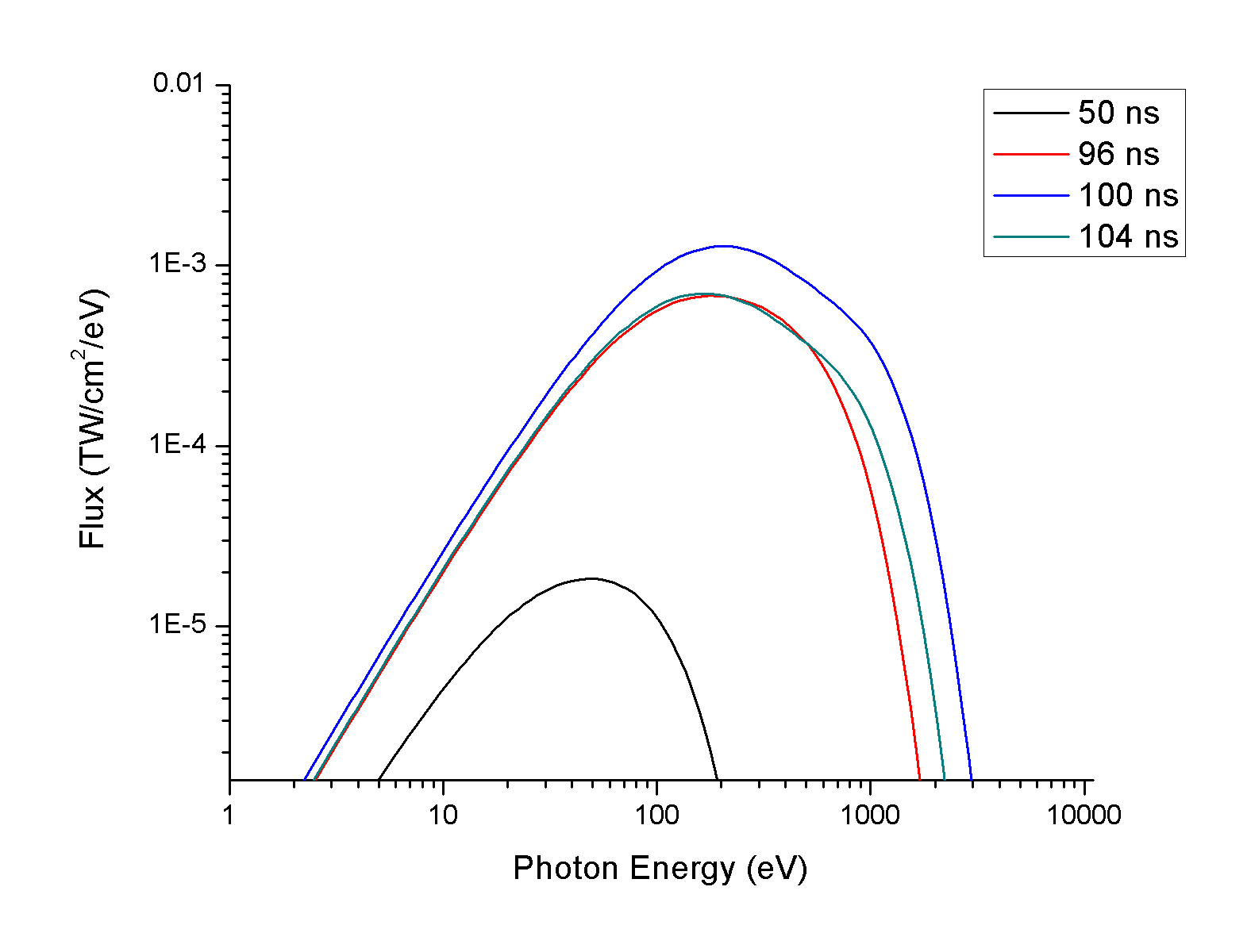
Time Evolution of Incident Spectrum on Center of Gas Cell |
An interesting feature of this plot is that the spectrum at 104 ns is very similar to the spectrum at 96 ns except for a lingering high energy tail in the spectrum for 104 ns. Since the power peak of the pinch is symmetric about 100 ns, one might think initially that the incident flux from the pinch on the gas cell should be similar at 96 and 104 ns. However, the radius of the pinch is NOT symmetric about 100 ns, such that the radius is much greater at 96 ns than it is at 104 ns. We know that since the pinch power is approximately the same at 96 and 104 ns,
Tem a
R-1/4 for a given flux,
where R is the radius of the pinch. Thus, if the radius is much smaller at 104 ns, the pinch will have a higher emission temperature, and thus will have a harder (or more energetic) emission spectrum. This explains the hard "bump" in the spectrum at t = 104 ns.
Next, we constructed a multigroup opacity model for the mylar in the windows of the gas cell. This model is only utilized in the hydrodynamics simulation if the mylar is labeled as a non-DCA (where DCA stands for Detailed Configuration Accounting) material. Since we had previously used for the mylar an opacity model for a plastic used in the witness plate of the halfraum for inertial confinement fusion (ICF) experiments, we thought it would be useful to make some plots comparing our new mylar opacity model to the old plastic model at several temperatures and densities.
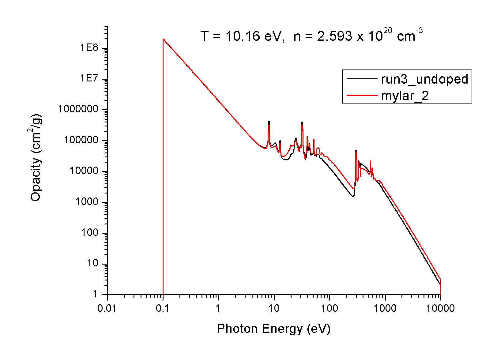
Comparison of the opacity of the mylar (red) and plastic (black)
|
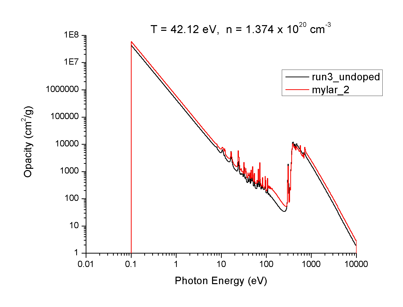
Comparison of the opacity of the mylar (red) and plastic (black)
|
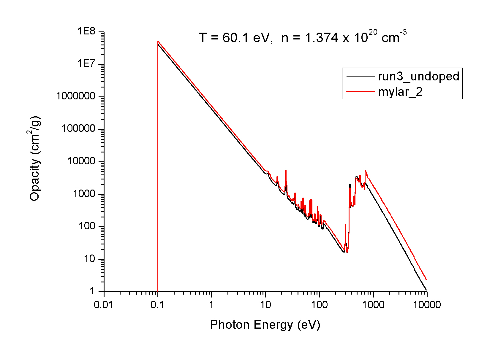
Comparison of the opacity of the mylar (red) and plastic (black)
|
In general we find that the mylar and witness plate plastic have very similar opacity curves, but when they do differ the mylar is more opaque than the witness plate plastic.
Using the DCA/non-DCA and LTE/NLTE options in Helios, we ran several
simulations with different options to see how changes in the materials
or the use of NLTE instead of LTE would affect the ion temperature and
mass density configuration. For non-DCA neon we created a multigroup
opacity table, and for DCA neon we created a DCA model for the neon by
selecting the ground state for all ionization stages except for
He-like (Ne IX) and H-like (Ne X) neon, for which we selected the
first 54 levels and all 22 levels respectively. Also, in an effort to
speed up the calculation, we used a configuration averaged model to
collapse the level populations for all ionization stages. For the DCA model,
the opacities were calculated at run time. We use a non-DCA model for mylar
in all of the simulations, so the multigroup opacity shown above is
used for each run. For the equations of state, we used the SESAME
files matr_07590_polystyrene.ses for the mylar and
matr_05410_neon.ses for the neon. Lastly, the incident
radiation flux at the face of the gas cell was inputted from a VisRad
output file.
First, we conducted a LTE simulation with the mylar and neon as non-DCA materials (use multigroup opacity models), and produced plots for the time dependent ion temperature and mass density as a function of position. NOTE: In the plots below, the incident radiation is impacting the gas cell from the left.
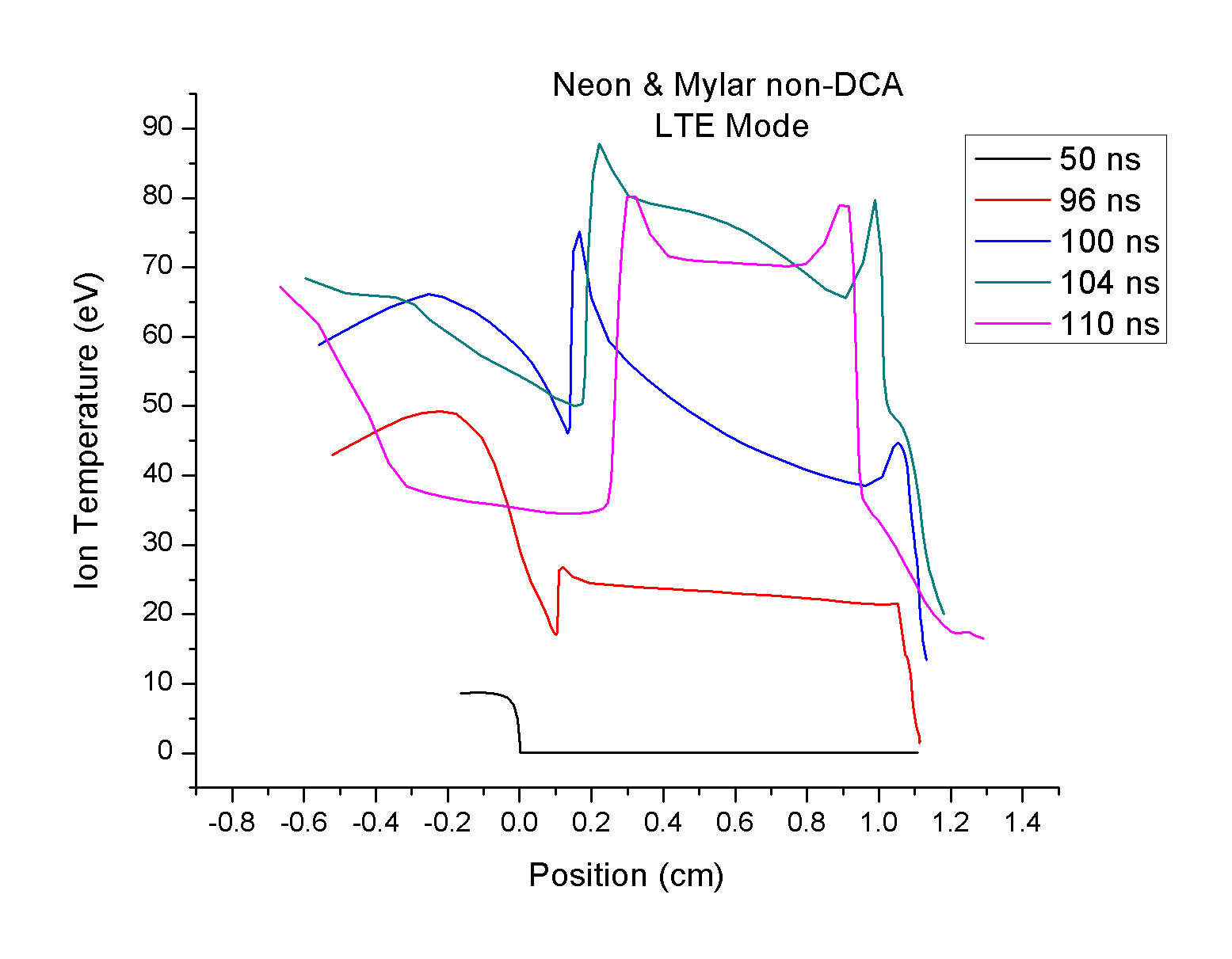
Ion Temperature vs. Position |
Mass Density vs. Position |
Ion Temperature vs. Position |
Mass Density vs. Position |
Finally, we ran a NLTE simulation with the mylar as a non-DCA material and the neon as a DCA material. The results are shown below.
Ion Temperature vs. Position |
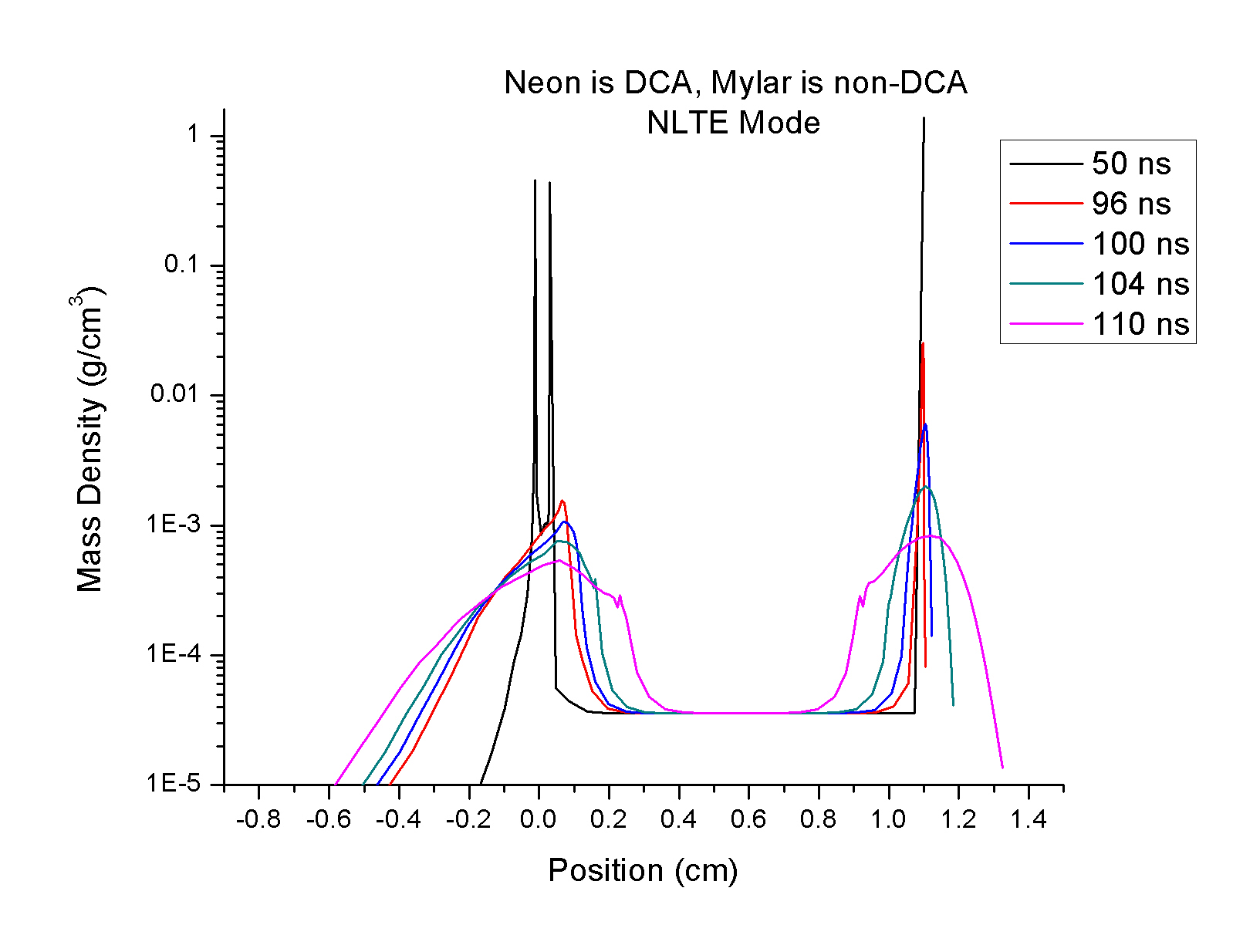
Mass Density vs. Position |
For this last simulation I also created a 3-D plot of the time dependent ion temperature as a function of position. See the plot below.
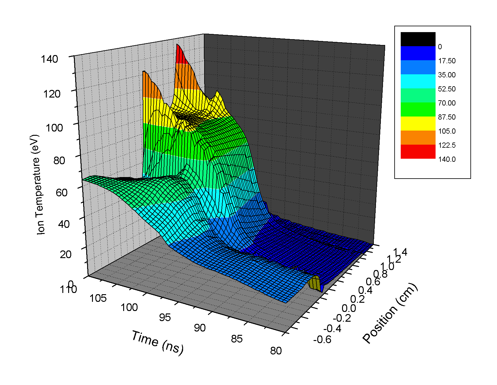
3-D Plot of Ion Temperature vs. Position |
Since the 3-D plot requires much more data in order to effectively grid the data into a matrix for 3-D plotting, this plot is much more complex than the other 2-D plots. With this plot, however, it is easier to visualize some concepts which are much more subtle or elusive in the 2-D plot. For example, for much of the climb to the plateu at 90 eV, the temperature gradient (which evidences the progression of a radiation wave) is present and progressing through the gas, but appears very weak.
In order to directly compare the results from the different simulations, I have also plotted the ion temperature and mass density as a function of position for one representative time (t = 100 ns, the peak of the pinch emission) for each simulation. See the plots below.
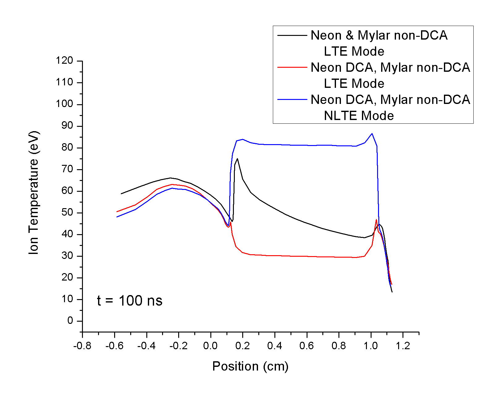
Ion Temperature vs. Position Comparison |
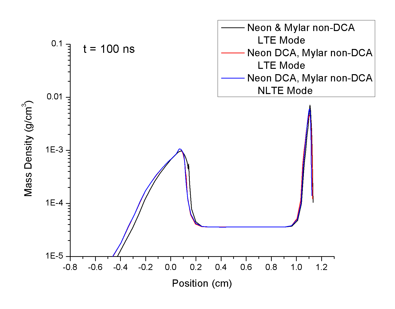
Mass Density vs. Position Comparison |
In the ion temperature plot, it is important to note (when compared to the LTE, non-DCA neon and mylar simulation) that if we keep LTE mode but make the neon a DCA material, the gas does not get as hot, but if we switch to NLTE mode, the gas becomes hotter. This clearly demonstrates that the NLTE mode makes a difference, and is evidence that the LTE approximation is not a good one.
The radiation wave (evidenced by the temperature gradient) occurs at later times (approximately 100 ns) in the LTE, non-DCA neon and mylar simulation than it does in either of the other two simulations. In fact, it appears that there is no radiation wave diffusing through the gas in the LTE, DCA neon and non-DCA mylar simulation, and the radiation wave in the NLTE, DCA neon and non-DCA mylar simulation is weak at best.
Not suprisingly, the mass density profiles for 100 ns are nearly identical since the mylar is a non-DCA material and therefore is not strongly affected by changes in the DCA status of the neon and whether we use LTE or NLTE mode. Things like changing the density of the gas fill or the thickness of the mylar windows are examples of factors which would noticeably change the mass density profile.
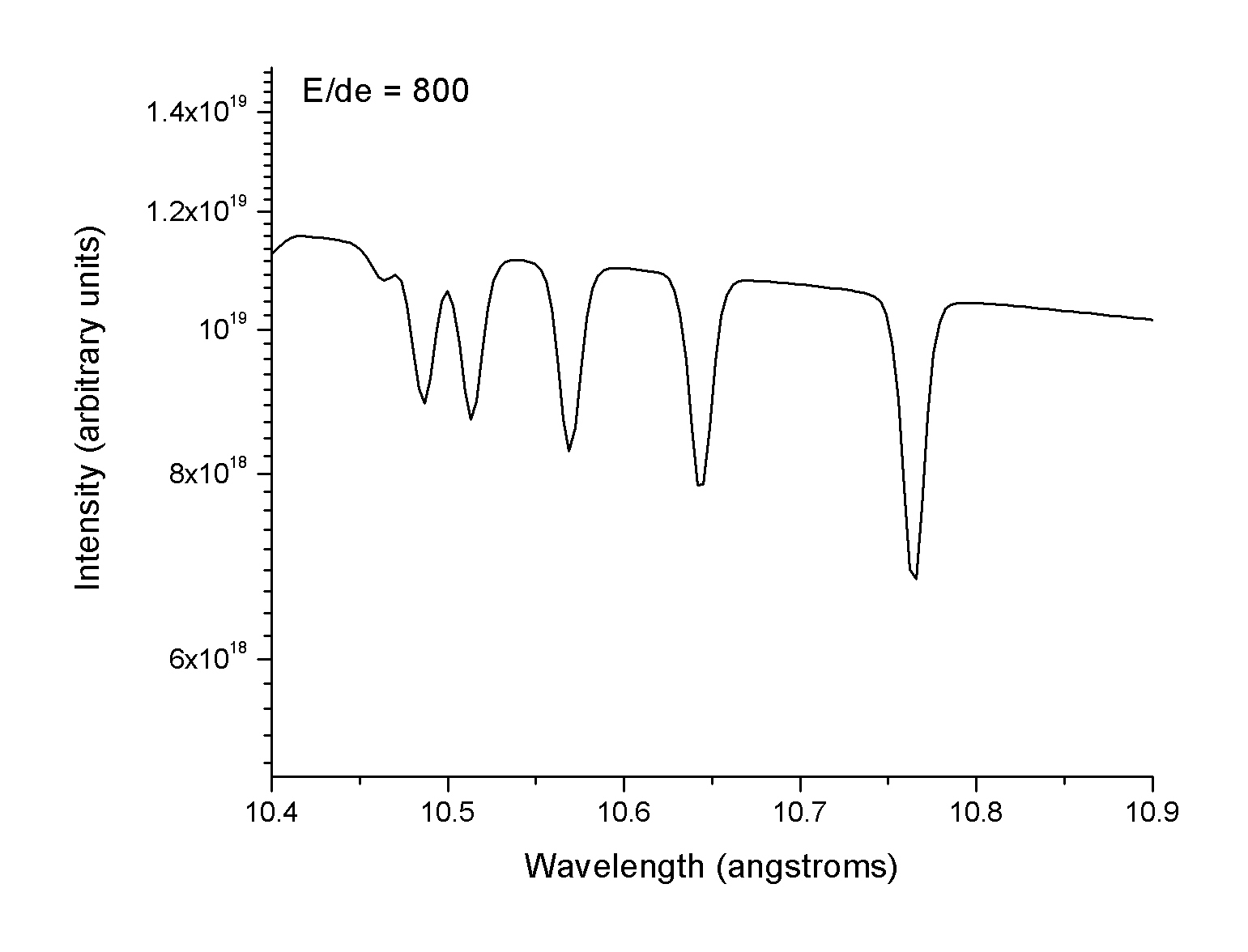
Using the hydrocode output file of the Helios NLTE, DCA neon and non-DCA mylar simulation, I synthesized several spectra using Spect3D. We thought it would be useful to compare our results to absorption spectra obtained in the actual experiments, so below I compare the synthesized spectra to a spectrum from Bailey et al. (2001) for shot Z543.
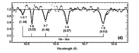
|
Figure taken from Bailey et al. (2001) |
|
LTE Kinetics Model DCA Opacities for Mylar and Neon Continuum Backlighter No External Radiation Field |
|
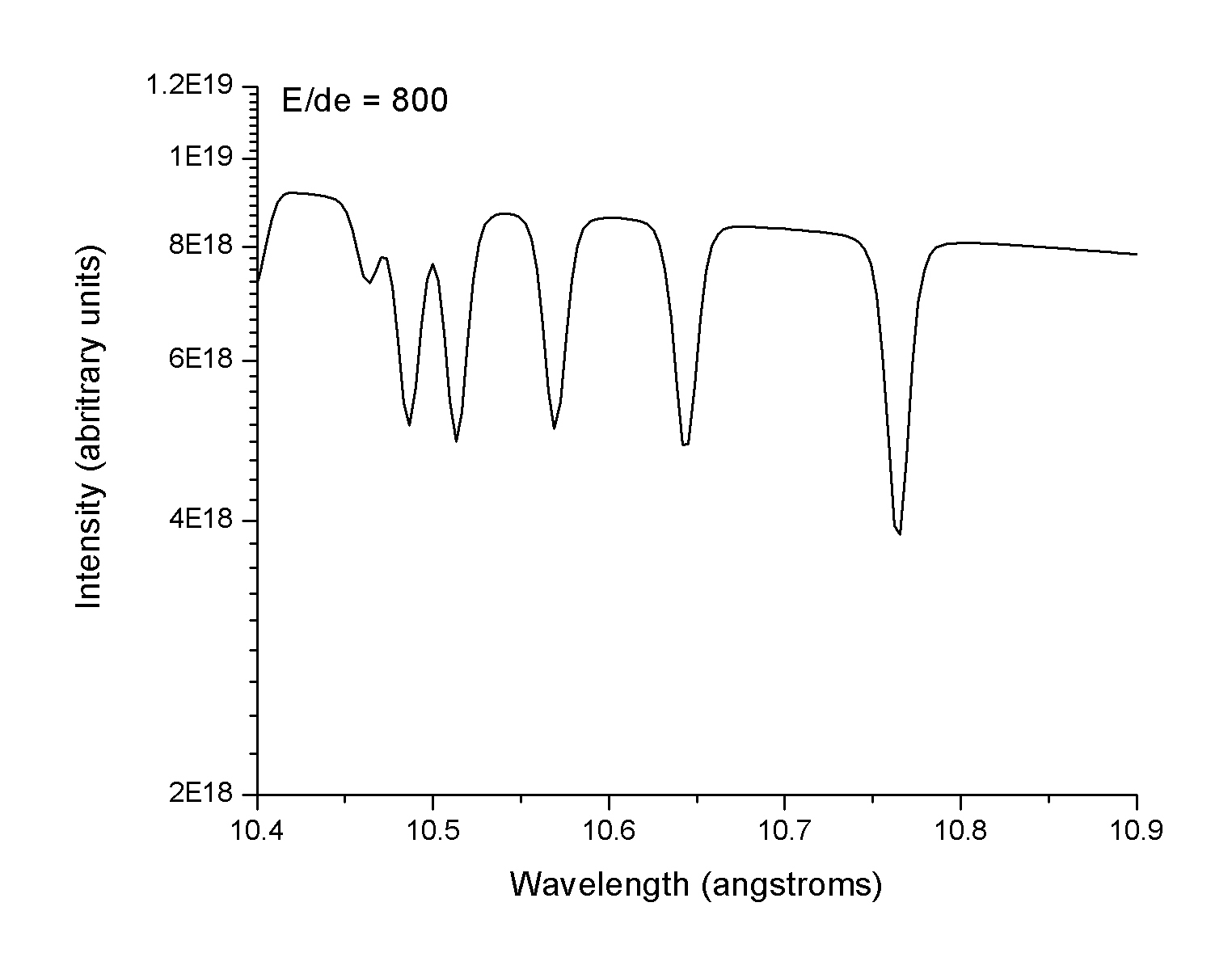
Collisional-Radiative Kinetics Model No Photoexcitation or Photoionization Model DCA Opacities for Mylar and Neon Continuum Backlighter No External Radiation Field |
|
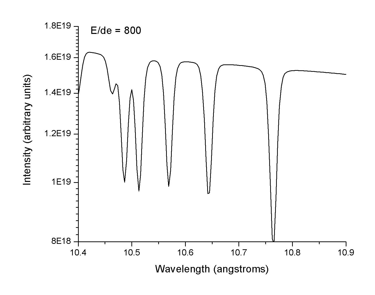
Collisional-Radiative Kinetics Model Non-Local Radiation Model for Photoexcitation and Photoionization DCA Opacities for Mylar and Neon Continuum Backlighter External Radiation Field (output of VisRad) |
Note that the spectral resolution for each of the three synthesized spectra is 800.
When we compare the synthesized spectra to the real spectra obtained from the gas cell experiment, we see that there is pretty good agreement in the absorption features. Though the profiles of the line are not identical, they do occur in the right number and right position in the spectrum. As we progressively move from LTE to NLTE (with an external radiation field), the absorption features get deeper.
By turning off the continuum backlighter in one of my Spect3D simulations, I obtained an emission spectrum for this same wavelength interval.
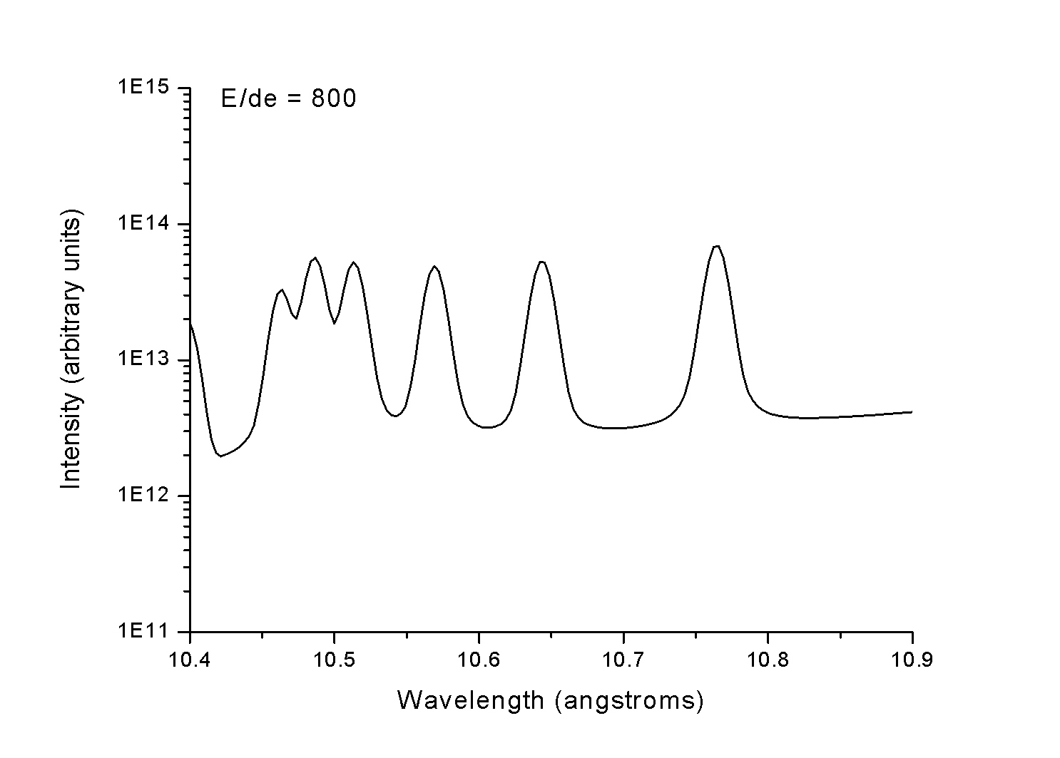
|
Collisional-Radiative Kinetics Model Non-Local Radiation Model for Photoexcitation and Photoionization DCA Opacities for Mylar and Neon NO Backlighter External Radiation Field (output of VisRad) |
Just as was the case for the absorption spectra, the spectral resolution for this spectrum is 800.