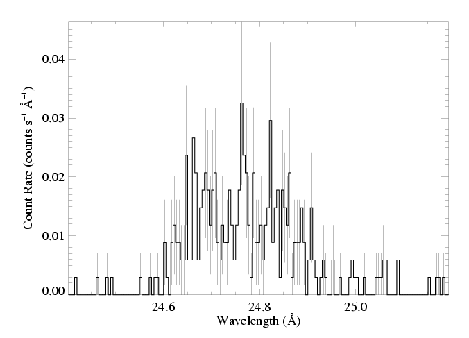
N VII 24.781 Angstroms
Models with isotropic porosity
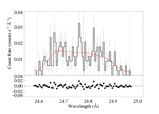
Note: We fit only the MEG data. There are 272 MEG counts in the spectral region we fit (and plot below). See the fitting log.
Same continuum fit as we used for the non-porous models: n=2, best-fit norm=2.13e-3. The 68% confidence limits on the normalization are +/- 5e-4. And the best fit is formally a good fit. View the spectral region near the line: MEG.

|
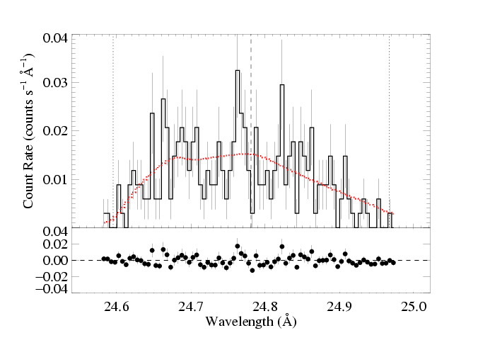
[24.58:24.98], λo = 24.781
vinf=2250 β=1 powerlaw continuum, n=2; norm=2.13e-3 q=0 hinf=93.3 +/- (11.5:99+) and for 90% confidence, (0.00:99+) taustar=28.5 +/- (4.5:99+) and for 90% confidence, (0.5:99+) uo=0.401 +/- (0.346:0.466) norm=7.62e-4 +/- (7.13e-4:8.13e-4) rejection probability = 70% (C=171.23; N=158) |
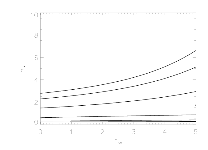
The important parameters, taustar and hinf, are essentially unconstrained. Some regions of parameter space are ruled out, as shown below. And uo is well constrained to be smaller than for other lines. But there's the whole issue of blending.
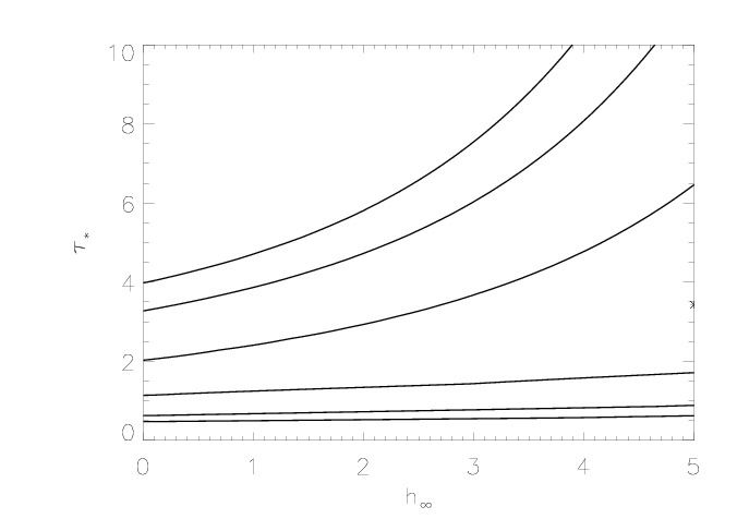
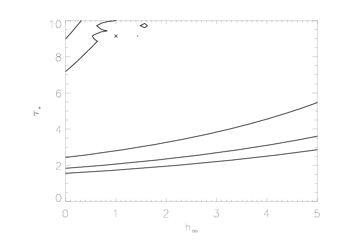
Here are the 68%, 90%, and 95% joint confidence limits on hinf and taustar. The asterisk represents the best-fit model, shown as the red histograms on the above plot.
|
Note that even though neither of these parameters is constrained individually, we can see that relatively high values of taustar are excluded for any reasonable value of the porosity length. Note also, that though low values of taustar (<4.5) are ruled out at the 68% level when we consider that parameter in isolation - see table above; when we consider the joint probability distribution of these two parameters, we can't rule out any value of taustar!
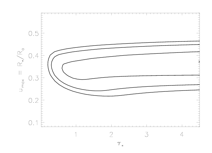
The confidence limits in taustar vs. uo expand in taustar when porosity is allowed, compared to the non-porous case, but the uo confidence limits are insensitive to taustar variations.
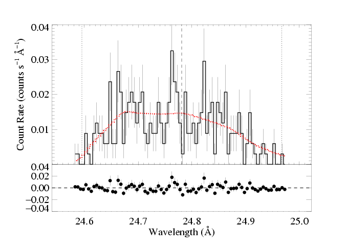
We examine the effects of blending here, too. We fit two wind profile models with parameters tied and normalizations scaled by 0.1 (N VI / N VII), and then 0.2 and 0.4. Here is the 0.1 case:
|
[24.58:24.98], λo = 24.781
vinf=2250 β=1 powerlaw continuum, n=2; norm=2.13e-3 q=0 hinf=16.6 +/- (7.0:99+) and for 90% confidence, (0.00:99+) taustar=37.3 +/- (4.5:99+) and for 90% confidence, (0.9:99+) uo=0.401 +/- (0.343:0.459) norm=7.02e-4 +/- (6.55e-4:7.50e-4); 0.1 for 2nd component rejection probability = 68% (C=172.46; N=158) |
The fit quality is a little worse, but still acceptable. The model parameter values and their uncertainties have not changed appreciably from the first fit, of the model with no blending with N VI assumed.
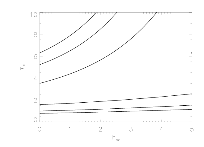
Here are the 68%, 90%, and 95% joint confidence limits on hinf and taustar. The asterisk represents the best-fit model, shown as the red histograms on the above plot.
|
Here is the 0.2 case:
|
[24.58:24.98], λo = 24.781
vinf=2250 β=1 powerlaw continuum, n=2; norm=2.13e-3 q=0 hinf=16.6 +/- (2.75:20.4) and for 90% confidence, (0.00:28.9) taustar=19.5 +/- (3.68:96.1) and for 90% confidence, (1.41:99+) uo=0.401 +/- (0.335:0.465) norm=6.48e-4 +/- (6.08e-4:6.93e-4); 0.2 for 2nd component rejection probability = 72% (C=174.58; N=158) |
Here are the 68%, 90%, and 95% joint confidence limits on hinf and taustar. The asterisk represents the best-fit model, shown as the red histograms on the above plot.
|
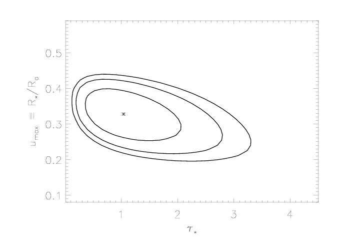
Here is the 0.4 case:
|
[24.58:24.98], λo = 24.781
vinf=2250 β=1 powerlaw continuum, n=2; norm=2.13e-3 q=0w hinf=2.02 +/- (0.00:8.5) and for 90% confidence, (0.00:14.1) taustar=6.78 +/- (3.07:28.6) and for 90% confidence, (2.28:70.0) uo=0.429 +/- (0.336:0.99) norm=5.62e-4 +/- (5.25e-4:5.99e-4); 0.4 for 2nd component rejection probability = 77% (C=178.58; N=158) |
Here are the 68%, 90%, and 95% joint confidence limits on taustar and uo. The asterisk represents the best-fit model, shown as the red histograms on the above plot.
|
Next, we fit isotropic porosity models to the data. And after that, anisotropic porosity models.
Back to main page.
last modified: 23 June 2008