Analysis Strategy

for the rest of the lines in the spectrum

Given the computational efficiency inherent in avoiding doing two integrals numerically, we will take beta=1 and for isotropic porosity, use the Rosseland bridging law. For anisotropic porosity, we have no choice but to do the double numerical integral (actually, we could use the "step" model, but we won't). However, for consistency sake, we will also take beta=1 and use the Rosseland bridging law in this case too.

So, for each line we will do the following:

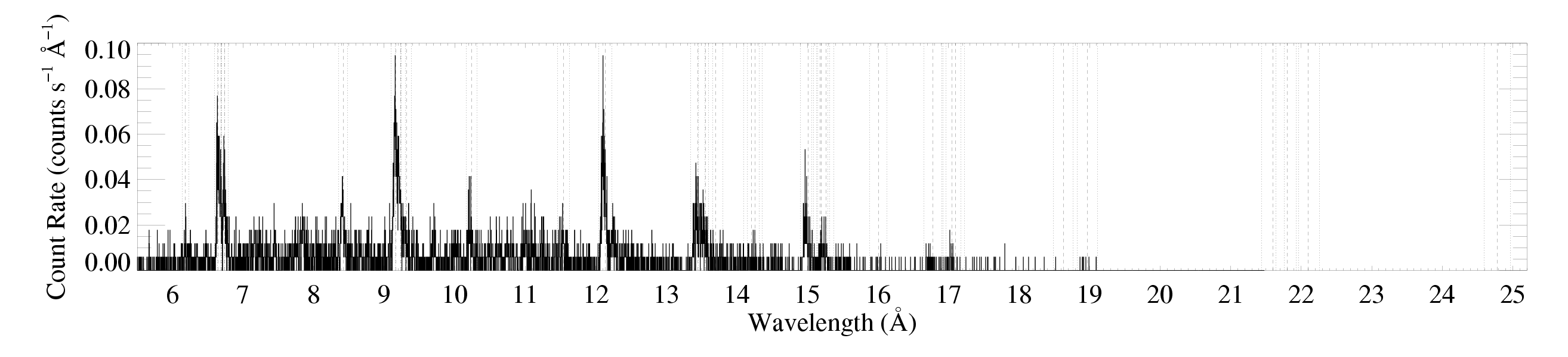
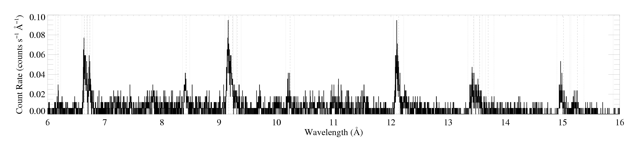
Assess (qualitatively; by visual inspection) whether it makes sense to include the HEG data in the fitting. Very large, detailed plots of the data are available on the main page (MEG, HEG: same wavelength range, and HEG: zoomed in on the region with strong lines).
Fit the continuum from a line free region near the line in question. We will generally make an attempt to quantify the uncertainty on the continuum level, but we've already shown that this won't make a significant difference in general.
Once we've settled on the data to use (MEG only or both gratings?) and established the continuum level, we'll keep these fixed, and determine the range over which to fit the line itself (from x=-1 to x=+1 with an epsilon added in each direction, unless concerns about line blending lead us to exclude some of this region.
We will then fit, in sequence: (1) a non-porous model (this should recapitulate the Kramer et al. (2003) results), including graphical 2-D confidence limits in taustar-u_o space, and also examine models where taustar is held fixed at the value implied by the literature mass-loss rate and our current model of atomic opacity in the wind (preliminary work from Zsargo & Hillier (Jan. 08)); (2) an isoporous model (this will include placing joint confidence limits on u_o and h_inf as well as on taustar and u_o), including forcing a model with taustar fixed at the value implied by the literature mass-loss rate and noting the constraints on h_inf in this case; and (3) repeating step 2 but with anisotropic porosity.

Then, to assess systematics - of a sort - we'll refit some of the lines using:

beta=0.8 (or, I suppose, we could use a specific value derived for the star in question).
And separately, we'll use the exponential (regular) opacity bridging law (and derive the constraints, especially, on h_inf for both iso and aniso porosity).

These two separate exercises will give us a sense of how much model assumptions affect the confidence limits on the important derived parameters.

Finally, we will explore the effects of the assumed terminal velocity on our results (especially the derived taustar values in the non-porous cases). We'll do this by refitting some (all?) of the lines in the non-porous case. We will selectively examine the two porous cases for a handful of lines too. We can bracket the adopted 2250 km/s standard terminal velocity assumption with 2200 km/s and 2350 km/s (Haser's dissertation).

Back to main page.

last modified: 27 April 2008