Exploring the effects of the continuum level
Determining the continuum level
We use the Fe XVII line at 15.014 Angstroms in the MEG as an example here.
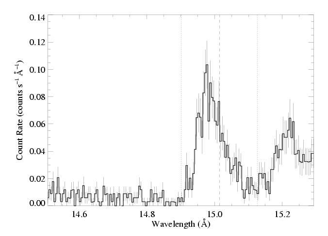
The emission line in question is centered at 15.014 - the vertical lines indicate the lab rest wavelength and the Doppler shifts associated with -/+ vinf. Note the weak, but non-zero, continuum on the blue side of the line. The true continuum is dominated by bremsstrahlung, but there are also weak emission lines blended in with the continuum. Some are in line lists and spectral models, while some are not. On the red side of the iron line is another complex of iron lines, centered around 15.26 Agstroms (but Doppler broadened and shifted too).
Fitting the continuum is not trivial, because of line blending. In general, we look for the lowest, or weakest, portion of the continuum near the line we want to fit, since blending with unidentified lines will only increase the apparent continuum level; it can never decrease it. (Of course, there are just as likely to be weak lines in the wavelength interval covered by the strong line as in any other portion of the spectrum; but still, we think the most conservative thing to do is pick portions of the spectrum that look least likely to be contaminated by unidentified lines, and fit a continuum model to those (small) portions.)
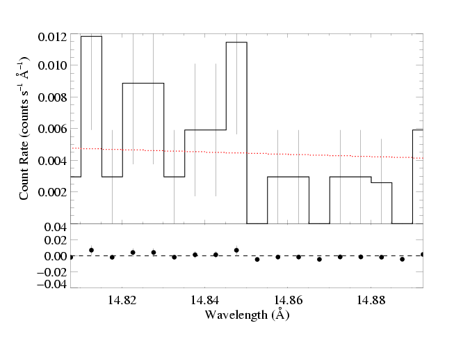
We fit a power law to the continuum, and fix its slope at n=2 (in ν-Fν space, which gives a flat continuum in λ-Fλ space). The wavelength range over which we're fitting is generally narrow enough that the slope is effectively flat. (Note that every model we show fit to data has been convolved with the response matrix, which accounts for broadening due to the finite resolution of the telescope/grating/detector assembly, and has been multiplied by the auxilliary response function, which represents the wavelength-dependent effective area. This latter function is not constant with wavelength, which is the reason the flat spectral model represented by the red line in the plot below does not look perfectly flat.)
|
n=2
norm=3.67e-3 +/- (3.01e-3:4.38e-3) Note: the uncertainties - or really 68% confidence range - on the continuum normalization level (which is in units of counts/s/Angstrom) are determined by the same ΔC criterion used to determine the confidence limits on the fit parameters of the wind-profile emission line model. |
Here we see that this portion of the continuum seems to contain some weak lines on the blue side. Looking back at the plot at the top of this page, we can see that there's effectively no portion of the spectrum redward of the line that isn't contaminated by other lines, so we fit only the continuum on the blue side. In general, though, we simultaneously fit regions on both sides of the line in order to establish the continuum level.
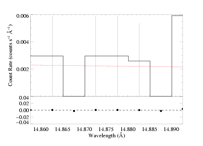
To avoid overestimating the continuum level due to the mistaken inclusion of weak lines on the blue side of the window shown above, we refit the model to just the very narrow range between 14.85 and 14.90. The fit is shown below.
|
n=2
norm=1.91e-3 +/- (1.26e-3:2.75e-3) |
In my opinion, this last fit - though it spans only a very small portion of the spectrum - is the most reliable measure of the continuum level; again, because it's much more likely that one overestimates the continuum by inadvertently including weak lines, than it is that one underestimates it (perhaps by focusing too much on statistical fluctuations; though, as mentioned above, there are likely weak lines blended with the line we're ultimately trying to fit, and so one could argue that the "continuum" model should account for these too). Perhaps we should conclude that the optimal continuum level to use should lie somewhere between these two values we've found, which differ by about a factor of two. Below, we explore the effects of choosing one or the other of these levels on the parameters derived from fitting the strong line at 15.014 Angstroms.
Exploring the effects on the line fit of the assumed continuum level
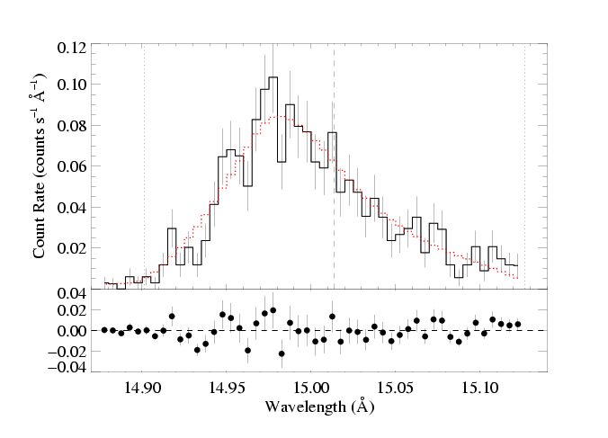
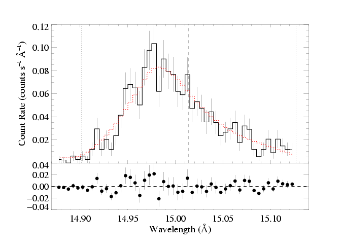
For the purposes of this exercise, we will fit the Fe XVII line at 15.014 in the MEG over the wavelength range [14.87:15.13] and assume a terminal velocity of 2250 km/s.
Here is the fit with the lower continuum level.
|
[14.87:15.13]
vinf=2250 β=1 powerlaw continuum, n=2; norm=1.91e-3 q=0 hinf=0 taustar=1.97 +/- (1.63:2.35) uo=0.655 +/- (0.605:0.725) norm=5.24e-4 +/- (5.04e-4:5.51e-4) rejection probability = 19% |
And here's the fit when we use the higher continuum level:
|
[14.87:15.13]
vinf=2250 β=1 powerlaw continuum, n=2; norm=3.67e-3 q=0 hinf=0 taustar=1.84 +/- (1.51:2.19) uo=0.668 +/- (0.618:0.729) norm=4.90e-4 +/- (4.72e-4:5.19e-4) rejection probability = 17% |
Note that the quality of the fit does not change (the C statistic value for these two fits differs by about 1). And the fit parameters hardly change at all (about 5% for taustar). The normalization of the line goes down when the continuum is stronger, as expected. But even this change is not significant for this strong line on top of a weak continuum. If you look at the left-most bins, in the bottom figure the model lies above the data (indicating that the continuum has been overestimated, though not unreasonably so), while the model fits these bins better in the upper plot).
Conclusions
The continuum level we choose is sensitive to the range over which it is determined. But in this example, varying the continuum level by a factor of ~2 leads to only very minor changes in the fitted model parameters.
Back to main page.
last modified: 22 April 2008