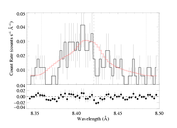
Mg XII 8.421 Angstroms
Models with anisotropic porosity
Note: Both MEG and HEG are being fit simultaneously
Same continuum fit as we used for the non-porous and isoporous models: n=2, best-fit norm=1.65e-3.
We use the "numerical" and "anisotropic" switches in windprofile. Note that the opacity bridging law is "regular" as opposed to Rosseland. Note: We have redone this analysis using the Rosseland opacity bridging law. That will be the considered the "official" anisoporous result. Note that we've also already explored the effects of opacity bridging law choice on our fiducial emission line at 15.014 Angstroms.
|
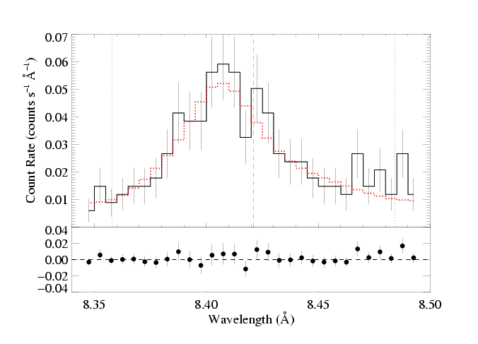
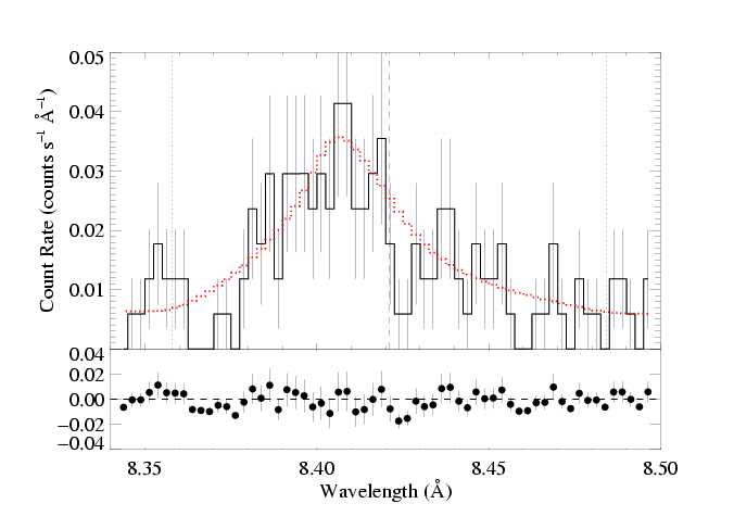
[8.34:8.50]
vinf=2250 β=1 powerlaw continuum, n=2; norm=1.65e-3 q=0 hinf=0.00 +/- (0.00:0.26) and for 90% confidence, (0.00:0.70) taustar=1.15 +/- (0.77:1.76) uo=0.734 +/- (0.661:0.875) norm=2.94e-5 +/- (2.72e-5:3.18e-5) rejection probability = 13% (C=186.52; N=188) |
Note that there's evidence for some of the same fit-robustness problems we saw with the isotropic porosity models, in that the confidence limits on the other wind parameters are tighter than we believe is realistic (in some cases, they're tighter than in the non-porous case, which doesn't make sense as that's a subset of this model family). In any case, we list the formal limits from the steppar command here, but they might be somewhat bigger. The confidence limit determination on the terminal porosity length, hinf, is robust, however.
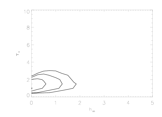
Here are the 68%, 90%, and 95% joint confidence limits on hinf and taustar based on fitting the MEG and HEG data together. The asterisk represents the best-fit model, shown as the red histograms on the above two plots.
|
The constraints are much tighter than in the isoporous case. Models with anisotropic porosity just don't give the right profile shapes. Also, smaller values of hinf have larger effects when clumps are flattened. Note that this grid doesn't have great resolution, it's only 20 by 20, because the run-time for numerically integrating the anisotropic model is quite long. But if need be, we can calculate a finer grid.
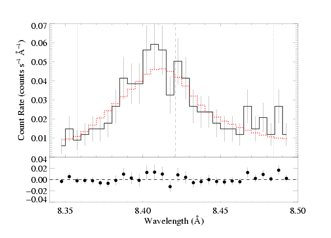
Forcing a fit with taustar=4:
|
[8.34:8.50]
vinf=2250 β=1 powerlaw continuum, n=2; norm=1.65e-3 q=0 hinf=1.46 +/- (0.85:2.75) and for 90% confidence, (0.62:4.46) taustar=4 uo=0.778 +/- (0.690:0.886) norm=3.06e-5 +/- (2.76e-5:3.26e-5) rejection probability = 27% (C=195.50; N=188) |
As the confidence limit contour plot, above, shows, this higher optical depth model is outside the 95% confidence range. In fact, it has ΔC~9, which implies that the non-porous model is preferred at the 99.7% level. And even so, very large terminal porosity lengths are required in order to accommodate taustar=4 (which is our estimate of the optical depth value implied by the literature mass-loss rate).
Back to main page.
last modified: 8 May 2008