ζ Pup: XMM RGS line-profile analysis

N VII at 20.910 A

There is almost no RGS2 data for this line, so we will use only the RGS1 data.

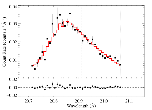
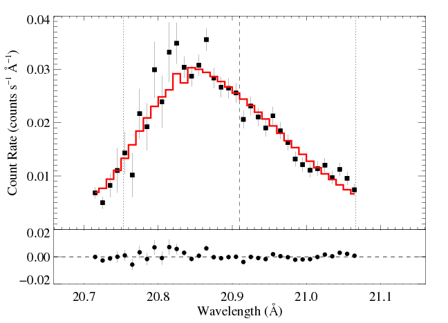
First we repeat the non-porous fit shown on the main page.

Non-porous: RGS1

[20.70:21.07] vinf = 2250 β = 1 powerlaw continuum, n = 2 norm = 9.05e-4   +/- (7.33e-4:1.13e-3) q = 0 hinf = 0 taustar = 4.93   +/- (3.90:5.59) Ro = 1.41   +/- (1.01:2.03) shift = 0 norm = 1.66e-4   +/- (1.56e-4:1.73e-3) chisq = 40.52 for N = 36

The fit is quite good (though mostly, I assume, because these data are relatively low S/N). The taustar value is high, as would be expected.

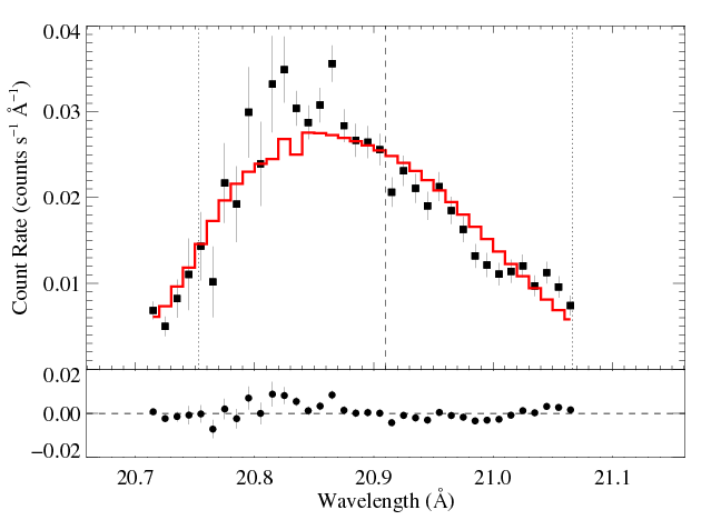
Next, we'll fit models with anisotropic porosity assuming flattened, radially oriented clumps. We use the "stretch" porosity length distribution, h(r), parameterized by h_inf. We will fit first with h_inf a free parameter, and then at fixed values of h_inf = 0.5, 1, 2, and 5 R_*.

aniso-porous: RGS1, h_inf free

[20.70:21.07] vinf = 2250 β = 1 powerlaw continuum, n = 2 norm = 9.26e-4   +/- (:) q = 0 hinf = 0.00   +/- (0.00:0.03) taustar = 4.88   +/- (4.00:5.89) Ro = 1.32   +/- (1.01:2.03) shift = 0 norm = 1.65e-4   +/- (1.56e-4:1.75e-4) chisq = 40.52 for N = 36

Note that despite the fact that the terminal porosity length's best-fit value is found to be zero (1e-7 or so, actually), the best-fit model parameters are not identical to the non-porous fit. They are very close, of course, but the small differences are probably due to the numerical integration that's required in the aniso case. Note that the 68% upper confidence limit on h_inf is 0.03, and that enables slightly larger confidence limits on taustar.

Now, a sequence of fits with fixed h_inf values of 0.5, 1, 2, and 5.

aniso-porous: RGS1, h_inf = 0.5

[20.70:21.07] vinf = 2250 β = 1 powerlaw continuum, n = 2 norm = 7.61e-4   +/- (5.26e-4:9.96e-4) q = 0 hinf = 0.5 taustar = 7.96   +/- (6.15:10.16) Ro = 1.60   +/- (1.24:2.01) shift = 0 norm = 1.69e-4   +/- (1.59e-4:1.80e-4) chisq = 52.92 for N = 36

aniso-porous: RGS1, h_inf = 1

[20.70:21.07] vinf = 2250 β = 1 powerlaw continuum, n = 2 norm = 6.20e-4   +/- (3.75e-4:8.79e-4) q = 0 hinf = 1 taustar = 12.95   +/- (9.61:17.46) Ro = 1.70   +/- (1.36:2.14) shift = 0 norm = 1.75e-4   +/- (1.63e-4:1.86e-4) chisq = 62.38 for N = 36

aniso-porous: RGS1, h_inf = 2

[20.70:21.07] vinf = 2250 β = 1 powerlaw continuum, n = 2 norm = 3.53e-4   +/- (:) q = 0 hinf = 2 taustar = 34.11   +/- (:) Ro = 1.62   +/- (:) shift = 0 norm = 1.86e-4   +/- (:) chisq = 73.45 for N = 36

aniso-porous: RGS1, h_inf = 5

[20.70:21.07] vinf = 2250 β = 1 powerlaw continuum, n = 2 norm = 3.53e-4   +/- (:) q = 0 hinf = 5 taustar = 100   +/- (:) Ro = 1.73   +/- (:) shift = 0 norm = 1.91e-4   +/- (:) chisq =84.35 for N = 36

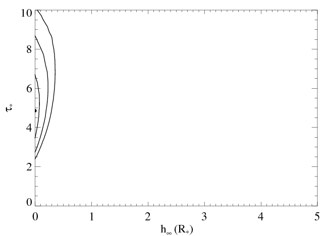
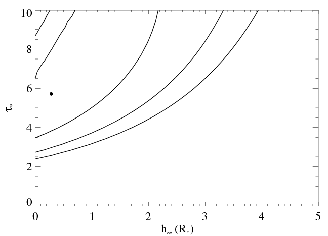
Summarizing

The effect of porosity and the tradeoff between porosity length and optical depth can be summarized by looking at the joint parameter confidence limits. We show the 68%, 95%, and 99% limits below. The best-fit model is the filled circle.

Now, we'll look at models with isotropic porosity.

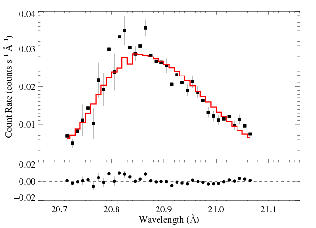
iso-porous: RGS1, h_inf free

[20.70:21.07] vinf = 2250 β = 1 powerlaw continuum, n = 2 norm = 9.11e-4   +/- (6.94e-4:1.14e-3) q = 0 hinf = 0.22   +/- (0.00:1.34) taustar = 5.55   +/- (3.90:9.18) Ro = 1.49   +/- (1.01:2.08) shift = 0 norm = 1.66e-4   +/- (1.56e-4:1.76e-4) chisq = 40.45 for N = 36

iso-porous: RGS1, h_inf = 0.5

[20.70:21.07] vinf = 2250 β = 1 powerlaw continuum, n = 2 norm = 9.19e-4   +/- (6.96e-4:1.11e-3) q = 0 hinf = 0.5 taustar = 6.18   +/- (4.72:8.07) Ro = 1.65   +/- (1.14:2.11) shift = 0 norm = 1.66e-4   +/- (1.56e-4:1.76e-4) chisq = 40.55 for N = 36

iso-porous: RGS1, h_inf = 1

[20.70:21.07] vinf = 2250 β = 1 powerlaw continuum, n = 2 norm = 9.19e-4   +/- (7.10e-4:1.15e-3) q = 0 hinf = 1 taustar = 7.42   +/- (5.51:10.09) Ro = 1.79   +/- (1.43:2.15) shift = 0 norm = 1.66e-4   +/- (1.56e-4:1.76e-4) chisq = 41.01 for N = 36

Note: with h_inf = 1, taustar has increased by 51 percent.

iso-porous: RGS1, h_inf = 2

[20.70:21.07] vinf = 2250 β = 1 powerlaw continuum, n = 2 norm = 9.40e-4   +/- (7.26e-4:1.16e-3) q = 0 hinf = 2 taustar = 10.16   +/- (7.40:14.42) Ro = 1.95   +/- (1.65:2.28) shift = 0 norm = 1.66e-4   +/- (1.56e-4:1.76e-4) chisq = 42.40 for N = 36

iso-porous: RGS1, h_inf = 5

[20.70:21.07] vinf = 2250 β = 1 powerlaw continuum, n = 2 norm = 8.39e-4   +/- (6.23e-4:1.06e-3) q = 0 hinf = 5 taustar = 26.09   +/- (18.13:38.53) Ro = 2.14   +/- (1.85:2.52) shift = 0 norm = 1.69e-4   +/- (1.60e-4:1.79e-4) chisq = 49.02 for N = 36

Summarizing

We show the 68%, 95%, and 99% limits below. The best-fit model is the filled circle.

And here is an extensive log of all these xspec fits.

 

Back to the top

---

last modified: 18 May 2012