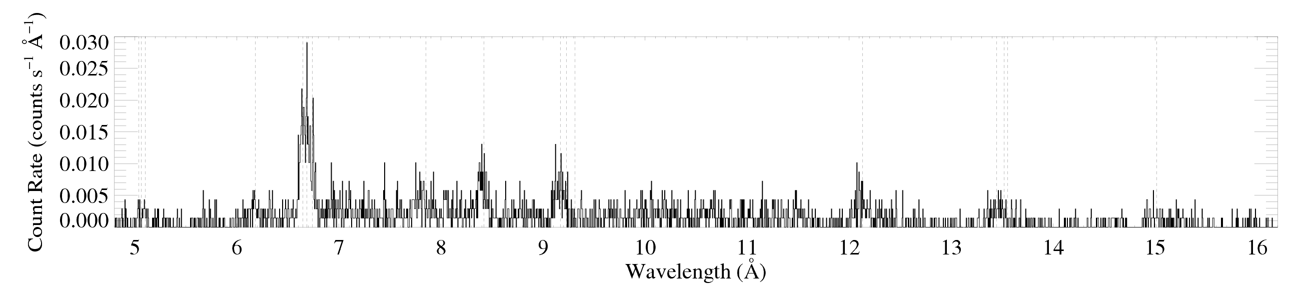
HD93129: Chandra grating spectrum

These plots are made from the 7 individual obs ids, reextracted and coadded by James MacArthur in July 2009. The combined exposure time is 139.5 ks (effective exposure time for the grating observations is 137.7 ks).

The HETGS spectra

MEG

HEG

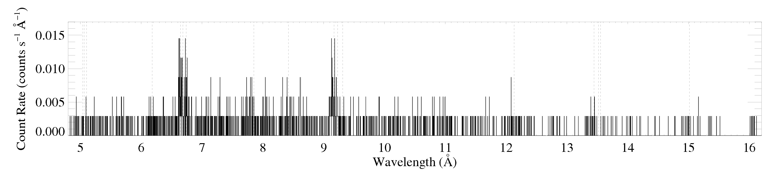
New: Note that in the manuscript, we show these data only up to 10 Angstroms [MEG and HEG].

Below, I reanalyze each line or line complex that has high enough signal-to-noise to justify analysis. (The Mg XI line at 7.85 can be fit, but the derived line flux is less than 2 sigma above zero, and so we do not include it. The Ne X line at 12.13 and a few other longer wavelength lines are contaminated (see next paragraph) and so they're not included in the analysis either.)

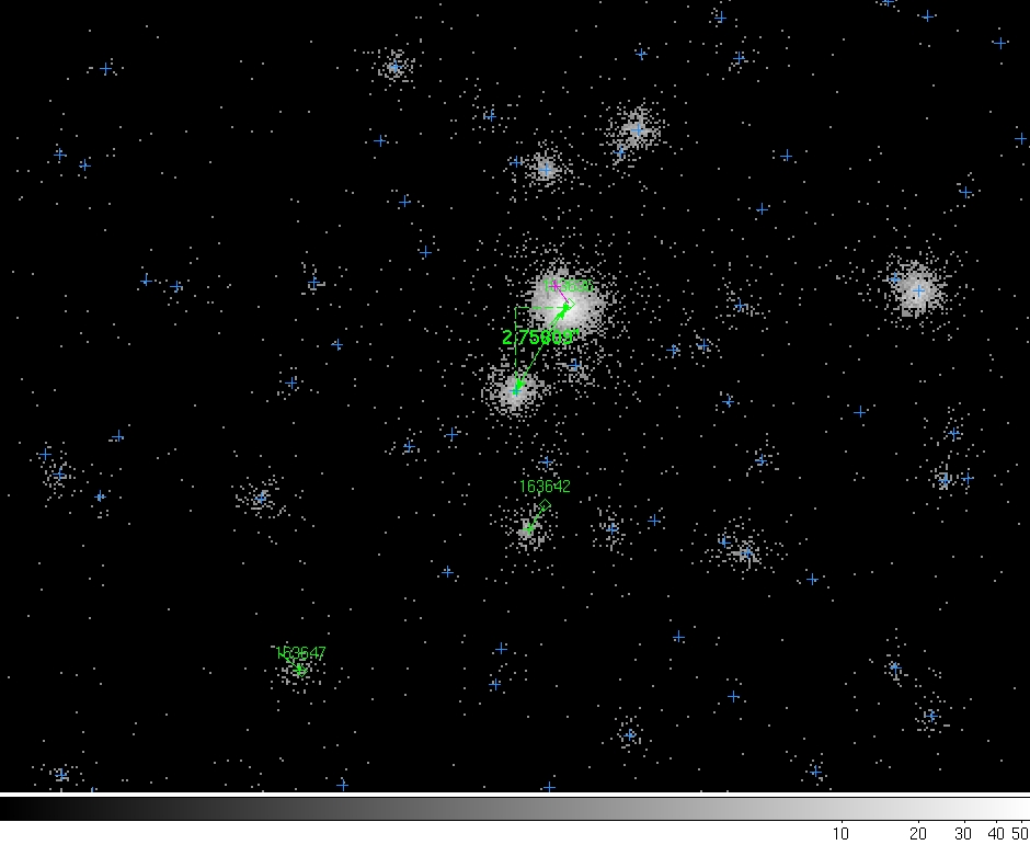
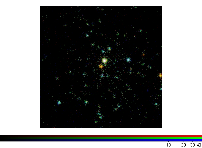
First, though, the reason for having to re-determine the zeroth order centroid position is the proximity of HD 93129B (2.8 or so arc seconds away), which can be seen in this image of the center of the ACIS detector (coadded seven Obs IDs). Component B is softer than A, as can be seen in this image in which the photon energy is color coded. And its flux is only about 10% that of component A. (The figure has been updated for the manuscript.) Both the lower flux and the softer emission can be seen quantitatively in the CCD spectral energy distribution of the zeroth order spectra. This figure indicates that contamination of the grating spectra should be negligible below about 10 Angstroms, but above that, there is likely to be mild contamination, and so we will not fit any lines longward of 10 Angstroms.

In the fits shown below, we have assumed v_inf=3200 and β=0.7 (Taresch et al.). However, we have also performed fits with two other values of the terminal velocity (3000 and 3400 km/s) for the strongest line in the spectrum (Mg XII Ly-alpha) and with β=1.0 (for every line). Note: Repolust et al. (2004) finds β = 0.8, but priv. comm. with J. Puls suggests that if clumping were included in the H-alpha analysis, a lower value of β would likely be found. So - for now - maybe β = 0.7 is the most reasonable estimate.

We start with the two isolated, Lyman-α lines, and then report on the He-like complexes.

8.4210 Angstroms: Mg XII

Here's β = 0.7

MEG HEG

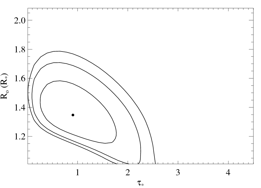
[8.32:8.54], λo = 8.4210 vinf=3200 β=0.7 powerlaw continuum, n=2; norm=2.12e-4 q=0 hinf=0 taustar=1.03   +/- (0.44:2.15)       (0.21:2.95) at 90% confidence Ro=1.44   +/- (1.17:1.71) norm=4.00e-6 +/- (3.53e-6:4.64e-6) rejection probability = ???% (C=217.07; N=260)

Here are the 68%, 90%, and 95% joint confidence limits on taustar and R_o. The filled circle represents the best-fit model, shown as the red histograms on the above plot.

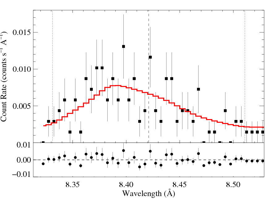
We also fit a model with β = 1.0.

Here are brief synopses of the fits to this line that assume different values of v_inf (default value 3200): v_inf=3000, β=1; v_inf=3400, β=1; and v_inf=3000, β=0.7; v_inf=3400, β=0.7.

Best-fit values for the different v_inf, β models:

taustar

	β = 0.7	β = 1.0
v = 3000	1.32	1.66
v = 3200	1.03	1.35
v = 3400	0.82	1.12

R_o

	β = 0.7	β = 1.0
v = 3000	1.51	1.94
v = 3200	1.44	1.81
v = 3400	1.39	1.73

This line -- the best S/N, unblended, uncontaminated line in the spectrum -- shows clear evidence of the characteristic skewed and blue-shifted profile from embedded wind shocks. Even allowing for a range of v_inf and β values, the non-zero, a value of taustar = 0 is excluded with > 90% confidence [visualization of β=0.7, v=3200 case].

Note that we tried allowing v_inf to be a free parameter, but its value is basically unconstrained (1870 to 4740 km/s is the 90% confidence range, while allowing the other physically meaningful model parameters to also be free).

To show in a somewhat less model-dependent way -- or at least using a more generic model -- the skewed and shifted profile properties, we fit a Gaussian profile to the line. First, with the Gaussian centroid fixed at the laboratory rest wavelength, and then with this parameter free. The width, σ, and normalization are free, and the Gaussian is superimposed on the same continuum model we used above, in fitting the wind-profile model.

wgauss + pow   MEG 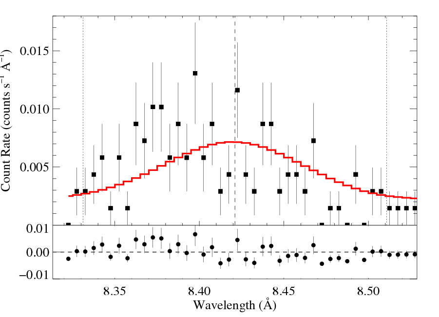HEG

[8.32:8.54], λo = 8.4210 powerlaw continuum, n=2; norm=2.12e-4 δ=0 σ=40.26   +/- (34.72:46.97) mA       (1434   +/- (1237:1673) km/s) norm=4.19e-6 +/- (3.51e-6:4.70e-6) rejection probability = ???% (C=228.73; N=260)

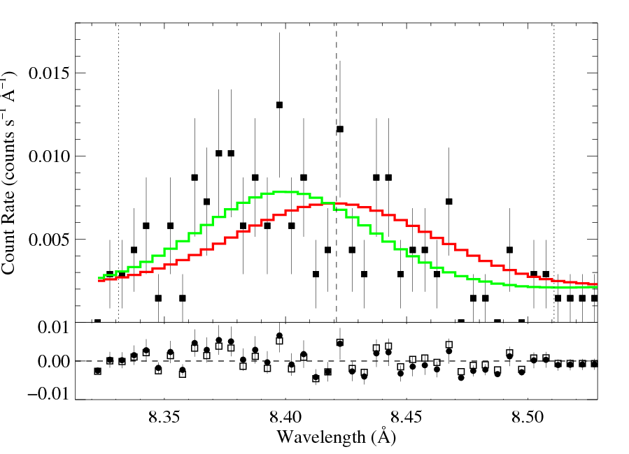
Now, with the centroid of the Gaussian free:

wgauss + pow   MEG 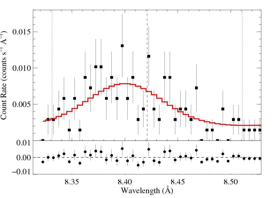HEG

[8.32:8.54], λo = 8.4210 powerlaw continuum, n=2; norm=2.12e-4 δ=-20.40   +/- (-25.99:-14.90) mA       (-727   +/- (-926:-531) km/s) σ=33.63   +/- (28.95:39.28) mA       (1198   +/- (1031:1399) km/s) norm=4.00e-6 +/- (3.49e-6:4.63e-6) rejection probability = ???% (C=216.90; N=260)

The unshifted Gaussian (with its centroid, δ, fixed at zero) provides a pretty poor fit: ΔC = 12, though there's one fewer free parameter than in the wind-profile model. This is strong evidence for a centroid shift, as expected from an embedded wind shock scenario. This is further confirmed in the second fit, where the centroid is allowed to be a free parameter and its value is significantly inconsistent with zero. But the fit quality is about as good as that found for the wind-profile model. So, the data aren't of good enough quality to distinguish the characteristic skewed profile shape from a generic (but blue-shifted) Gaussian shape, although the data are certainly consistent with the characteristic skewed profile shape. See an updated figure, showing both Gaussian models, that we're now including in the manuscript.

What about porosity?

We refit the wind profile model (with β=0.7 and v=3200) but fixed taustar at 4.2, with is the value expected for a mass-loss rate of 1.8 X 10^-5 M_sun/yr and an opacity of κ=23 at 8.4 Angstroms. We allowed the terminal porosity length, h_inf, to be a free parameter (the clumps are assumed to be spherical - "isotropic porosity"), where the local porosity length scales as h = h_inf(1 - R_star/r)^β.

MEG HEG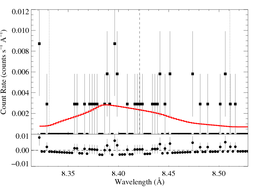

[8.32:8.54], λo = 8.4210 vinf=3200 β=0.7 powerlaw continuum, n=2; norm=2.12e-4 q=0 hinf=5.26   +/- (2.45:10.8) taustar=4.2 Ro=1.40   +/- (1.24:1.60) norm=4.18e-6 +/- (3.55e-6:4.63e-6) rejection probability = ???% (C=217.00; N=260)

So, the fit is as good as those from non-porous models, but the terminal porosity length is h_inf = 5.3 R_star (with a 68% lower confidence limit of 2.5 R_star).

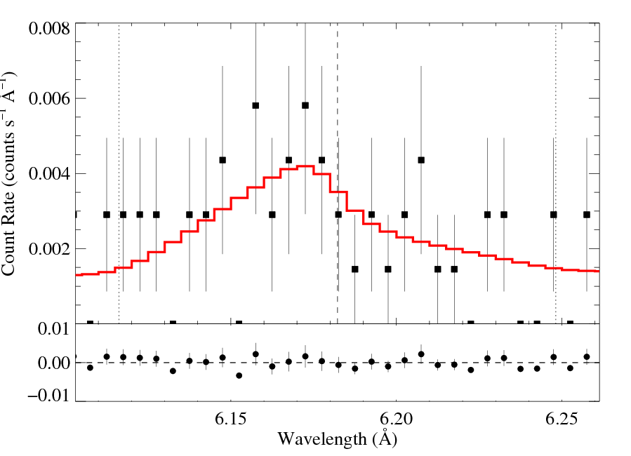
6.1822 Angstroms: Si XIV

Here's β = 0.7

MEG	[6.09:6.27], λo = 6.1822 vinf=3200 β=0.7 powerlaw continuum, n=2; norm=1.64e-4 q=0 hinf=0 taustar=1.64   +/- (0.38:3.44)       no constraints (0:100) at 90% confidence Ro=1.01   +/- (1.01:1.53) norm=1.48e-6 +/- (1.07e-6:1.97e-6) rejection probability = ???% (C=70.60; N=70)

Here are the 68%, 90%, and 95% joint confidence limits on taustar and R_o. The filled circle represents the best-fit model, shown as the red histograms on the above plot.

Note the marginal quality of these data renders the precision of the derived model parameters quite marginal as well.

Note also that due to the very low signal, we exclude the HEG data from the fitting.

We also fit a model with β = 1.0.

The next three line complexes are all He-like:

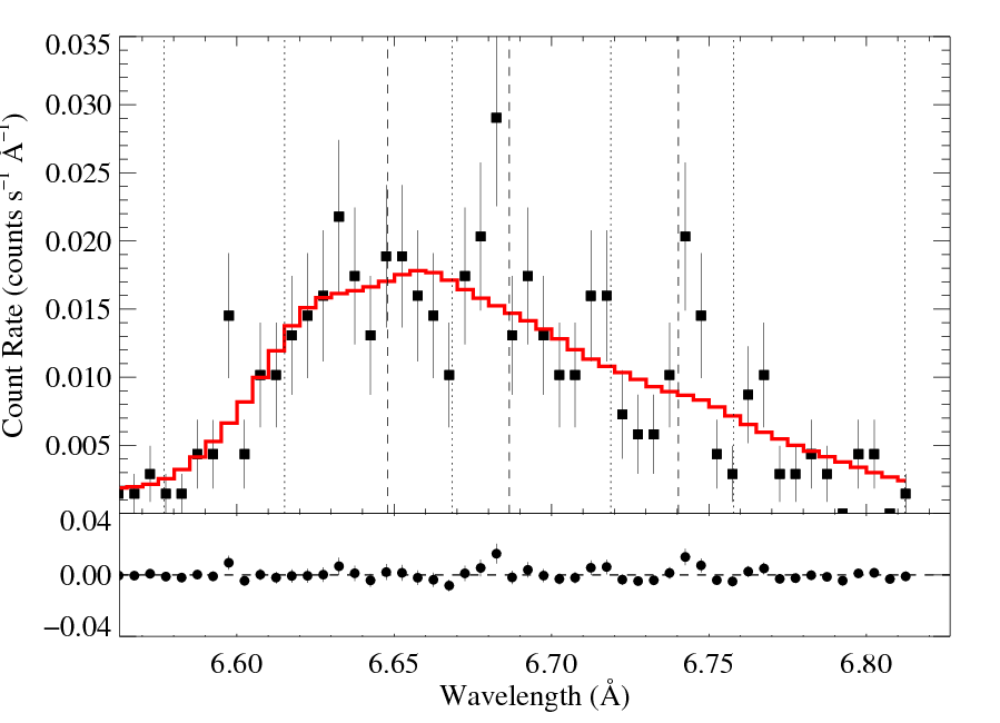
6.6479, 6.6866, 6.7403 Angstroms: Si XIII

Details of photoexcitation modeling.

Here's β = 0.7

MEG HEG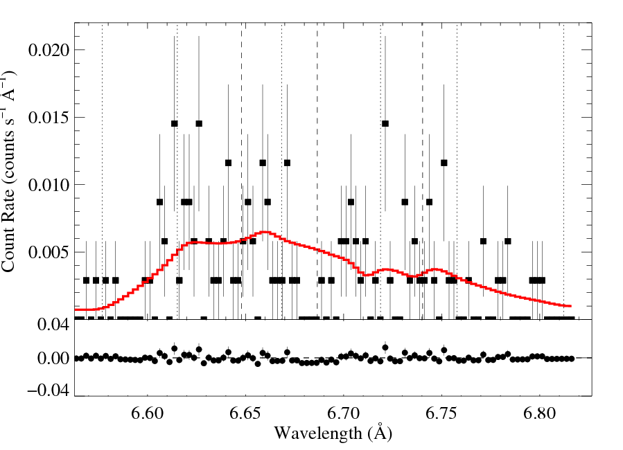

[6.56:6.82], λo = 6.6479, 6.6866, 6.7403 vinf=3200 β=0.7 powerlaw continuum, n=2; norm=1.83e-4 q=0 hinf=0 taustar=0.81   +/- (0.42:1.44) Ro=1.37   +/- (1.23:1.49) G=1.18   +/- (0.98:1.44) φ-ratio = 17   norm=1.68e-5 +/- (1.60e-5:1.79e-5) rejection probability = ???% (C=317.10; N=308)

Here are the 68%, 90%, and 95% joint confidence limits on taustar and R_o. The filled circle represents the best-fit model, shown as the red histograms on the above plots.

We also fit a model with β = 1.0. Note that the β = 1.0 fit is marginally preferred over the β = 0.7 fit (ΔC = 2.1)

For a more empirical look at this He-like complex, we fit a three-Gaussian model:

MEG HEG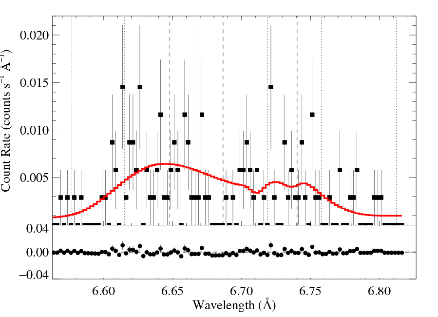

[6.56:6.82], λo = 6.6479, 6.6866, 6.7403 powerlaw continuum, n=2; norm=1.83e-4 R = f/i=1.12   +/- (0.85:1.51)       constraints at 90% confidence: (0.72:1.89) Note: "low density limit (Ro)" = 2.3 G=1.31   +/- (1.02:1.68) σv=1109 +/- (998:1232) km/s δv=-603 +/- (-770:-428) km/s norm=1.69e-5 +/- (1.59e-5:1.78e-5) rejection probability = ???% (C=315.38; N=308)

So, the f/i ratio is low, as we'd expect from plasma close to the photosphere (and consistent, qualitatively, with the results from the windprofile fits. The inconsistency of the fitted f/i value (at > 90% confidence) with the "low density limit" of 2.3 (which is what you'd get in a wind-wind shock zone far from the star(s)'s photosphere(s)) is further confirmation that (the bulk of) the X-rays are formed in embedded wind shocks.

To look at this a little further, we fit another three Gaussian model, but one where f/i = 2.3 is fixed.

MEG HEG

[6.56:6.82], λo = 6.6479, 6.6866, 6.7403 powerlaw continuum, n=2; norm=1.83e-4 R = f/i=2.3 G=0.96   +/- (0.75:1.21) σv=1179 +/- (1078:1288) km/s δv=-530 +/- (-712:-336) km/s norm=1.71e-5 +/- (1.60e-5:1.79e-5) rejection probability = ???% (C=319.87; N=308)

The low f/i value is preferred at >95% confidence. But note also that the intercombination line looks somewhat centrally peaked. Could this be contamination from wind-wind X-rays? Most likely, it's just statistical...

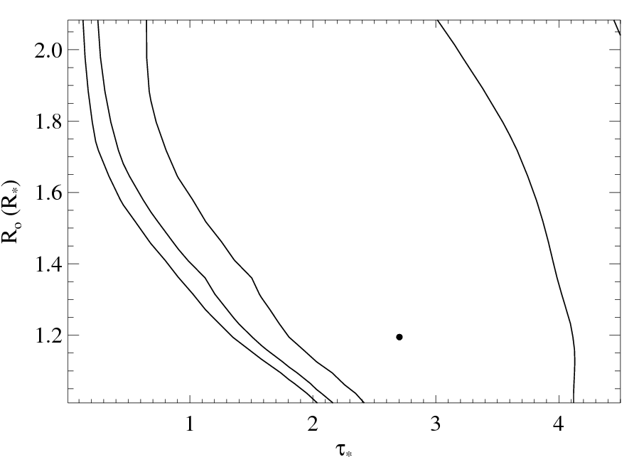
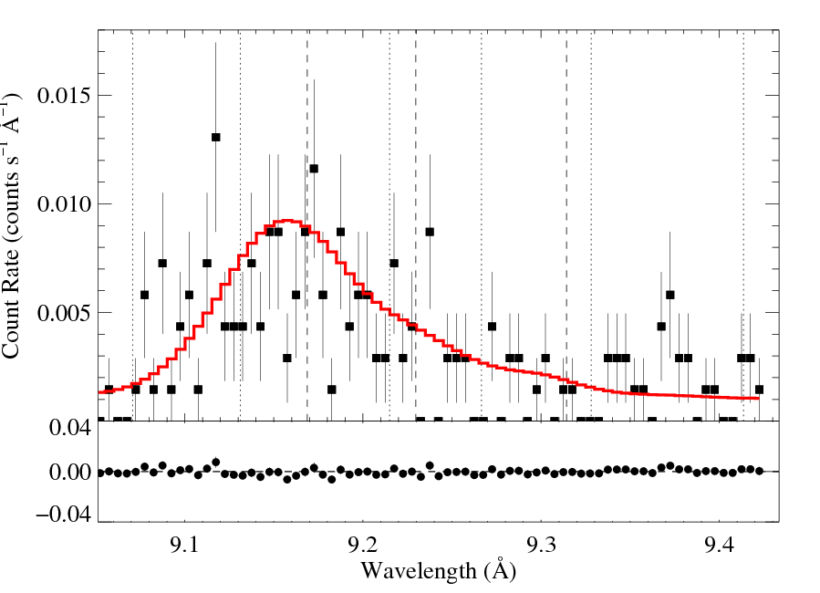
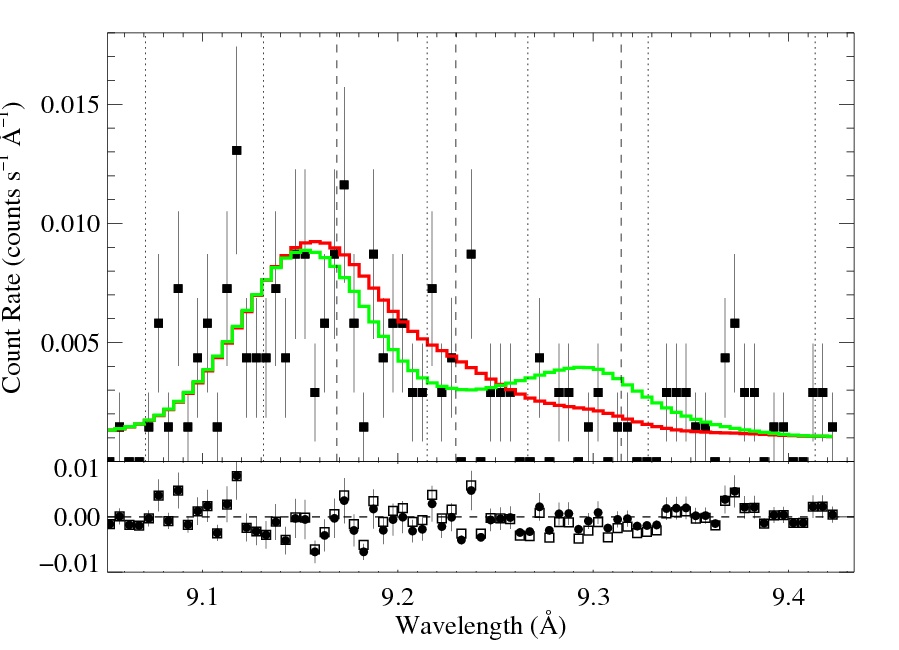
9.1687, 9.2297, 9.3143 Angstroms: Mg XI

Details of photoexcitation modeling.

Here's β = 0.7

MEG HEG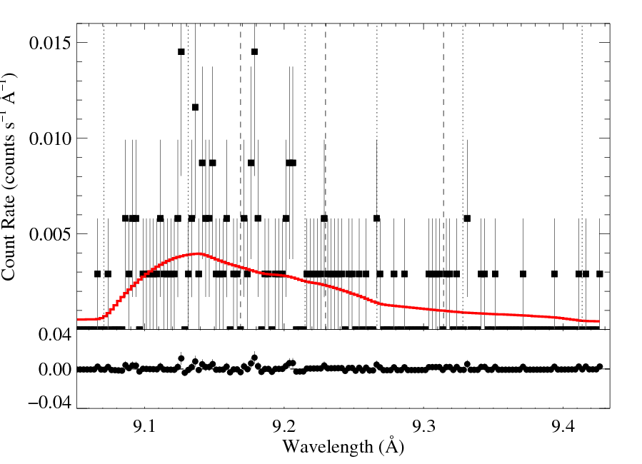

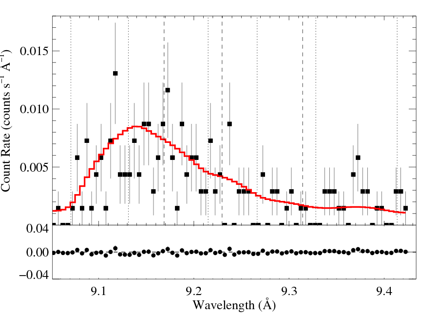
[9.04:9.43], λo = 9.1687, 9.2297, 9.3143 vinf=3200 β=0.7 powerlaw continuum, n=2; norm=2.05e-4 q=0 hinf=0 taustar=2.84   +/- (1.15:3.56)       0.54:4.30 at 90% confidence Ro=1.20   +/- (1.01:2.08) G=0.51   +/- (0.32:0.66) φ-ratio = 147   norm=1.61e-5 +/- (1.47e-5:1.72e-5) rejection probability = ???% (C=411.60; N=464)   fit log

Here are the 68%, 90%, and 95% joint confidence limits on taustar and R_o. The filled circle represents the best-fit model, shown as the red histograms on the above plots.

Here the best-fit G value is pretty small (though not completely unreasonably so). And so we also show a fit for which we froze G at 0.71, the value expected from atomic physics at the temperature of peak emissivity.

We also fit a model with β = 1.0.

As we did for the higher S/N Si XIII complex, above, for a more empirical look at this He-like complex, we fit a three-Gaussian model:

But here, we found far too much degeneracy among the model parameters. Specifically, with all parameters free, G gets small (so the f and i lines are very weak) and the width parameter gets very big -- apparently so the blended r and i lines can be fit by a single, broad Gaussian. Therefore, we choose to fix the width and shift parameters at the values found from fitting the Si XIII complex; and also fix G = 0.71.

MEG HEG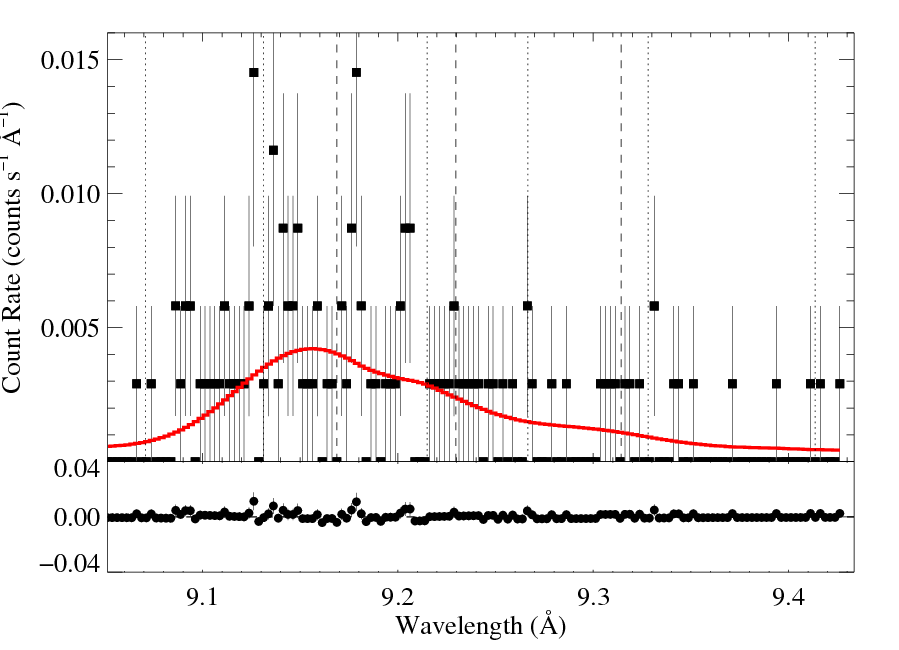

[9.04:9.43], λo = 9.1687, 9.2297, 9.3143 powerlaw continuum, n=2; norm=2.05e-4 R = f/i=0.40   +/- (0.23:0.63)       constraints at 90% confidence: (0.14:0.83) Note: "low density limit (Ro)" = 2.7 G=0.71 σv=1100 km/s δv=-600 km/s norm=1.58e-5 +/- (1.42e-5:1.68e-5) rejection probability = ???% (C=425.16; N=464)

So, the f/i ratio is low, as we'd expect from plasma close to the photosphere (and consistent, qualitatively, with the results from the windprofile fits. The inconsistency of the fitted f/i value (at > 95% confidence) with the "low density limit" of 2.7 (which is what you'd get in a wind-wind shock zone far from the star(s)'s photosphere(s)) is further confirmation that (the bulk of) the X-rays are formed in embedded wind shocks. This result is consistent with what we find for the Si XIII complex.

To look at this a little further, we fit another three Gaussian model, but one where f/i = 2.7 is fixed.

MEG HEG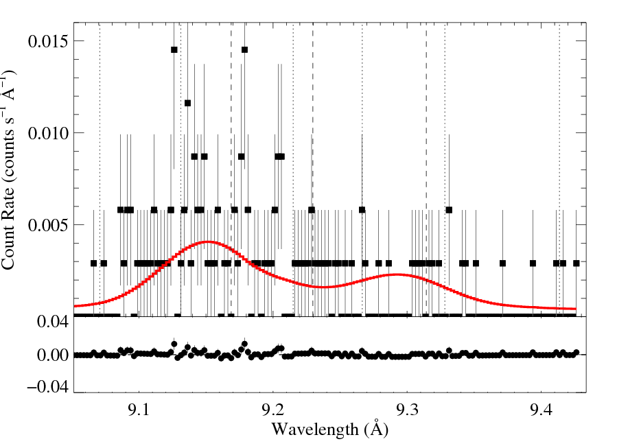

[9.04:9.43], λo = 9.1687, 9.2297, 9.3143 powerlaw continuum, n=2; norm=2.05e-4 R = f/i=2.7 G=0.71 σv=1100 km/s δv=-600 km/s norm=1.62e-5 +/- (1.50e-5:1.74e-5) rejection probability = ???% (C=442.70; N=464)

The low f/i value is preferred at >95% confidence.

See an updated figure, showing both Gaussian f/i models, that we're now including in the manuscript.

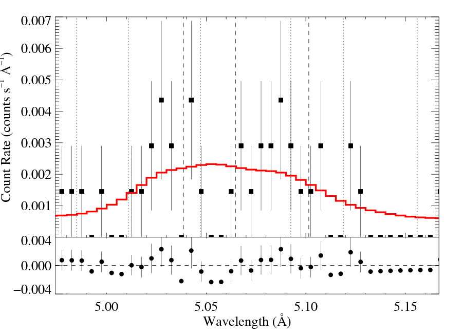
5.0387, 5.0648, 5.1015 Angstroms: S XV

Here, the S/N is quite low; to get a significant result (normalization 3σ above zero), we had to restrict ourselves to the MEG data, only. We also did not do detailed atmosphere modeling for the UV flux, we simply used a value of φ_ratio scaled up modestly from the ζ Pup value, in line with what our detailed calculations show for Mg XI and Si XIII.

Here's β = 0.7

MEG	[4.90:5.20], λo = 5.0387, 5.0648, 5.1015 vinf=3200 β=0.7 powerlaw continuum, n=2; norm=2.14e-4 q=0 hinf=0 taustar=0.54   +/- (0.00:2.03) Ro=1.18   +/- (1.01:1.69) G=1.85   +/- (0.85:5.07) φ-ratio = 4.0   norm=4.26e-6 +/- (3.20e-6:5.45e-6) rejection probability = ???% (C=104.14; N=118)   fit log

We tried a model where the G ratio was frozen at G = 0.7. The results were not significantly different; taustar = 0.32 with a 68% upper limit of 1.68. The R_o range didn't change that much.

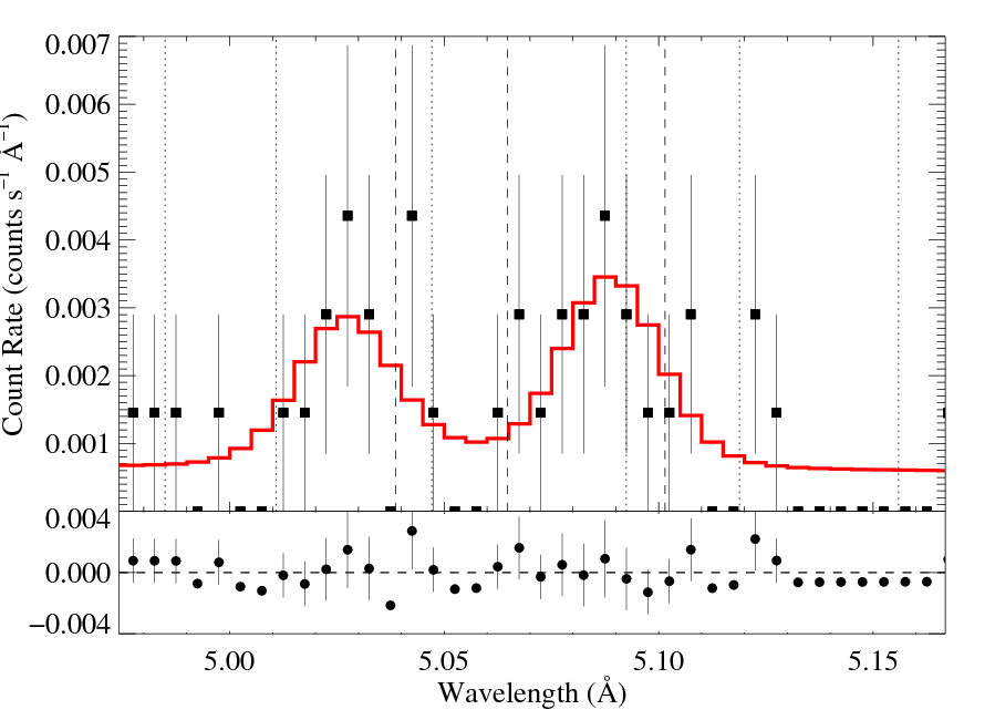
Next, hegauss fits:

Allowing R = f/i to be a free parameters leads to very high values of R.

MEG	[4.90:5.20], λo = 5.0387, 5.0648, 5.1015 powerlaw continuum, n=2; norm=2.14e-4 R = f/i = 20   +/- (2.86:unconstr.) G=1.39   +/- (0.83:2.75) σv = 493 km/s   +/- (192:773) δv = -692 km/s   +/- (-942:-452) norm=4.15e-6 +/- (3.12e-6:5.55e-6) rejection probability = ???% (C=99.28; N=118)

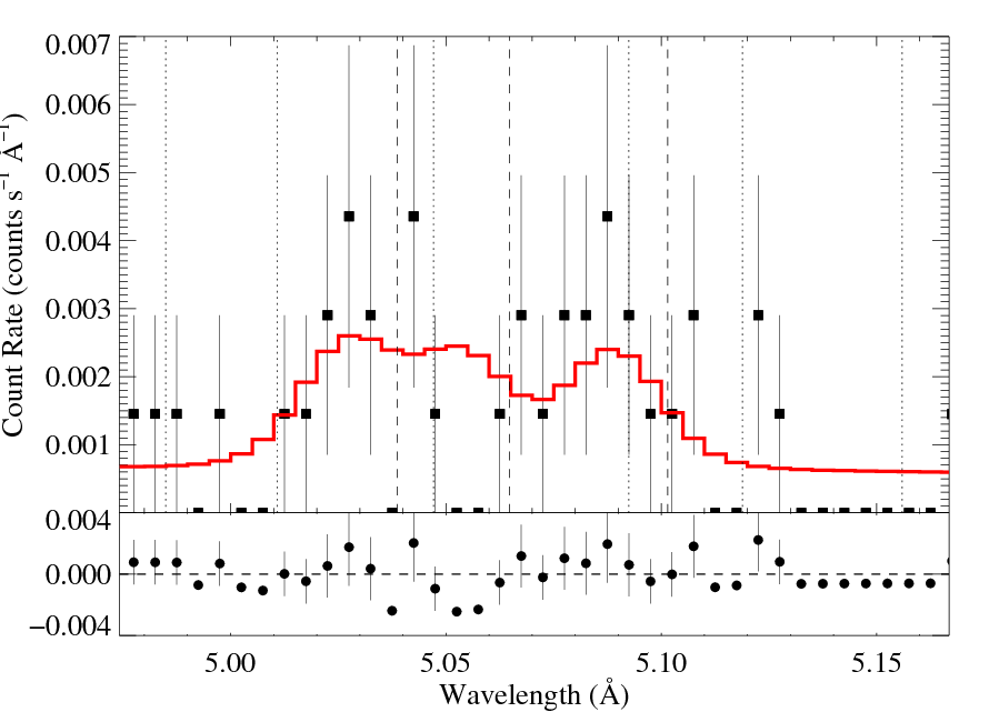
This very high value of R is not realistic. Let's look at the lowest value of R that's consistent with the fit. The 95% lower confidence limit is R = f/i = 1.08:

MEG	[4.90:5.20], λo = 5.0387, 5.0648, 5.1015 powerlaw continuum, n=2; norm=2.14e-4 R = f/i = 1.08 G=1.90   +/- (0.98:4.56) σv = 472 km/s   +/- (69:1046) δv = -688 km/s   +/- (-1068:-237) norm=4.02e-6 +/- (3.03e-6:5.22e-6) rejection probability = ???% (C=103.02; N=118)

 

Results

Mass-loss rate determination

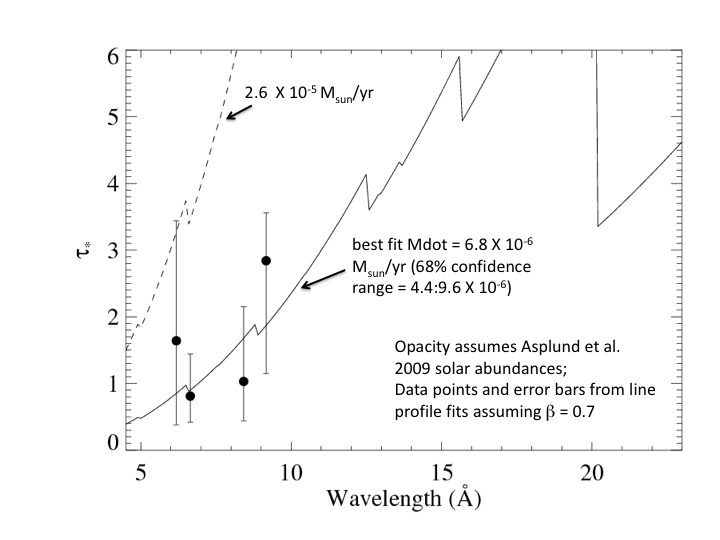
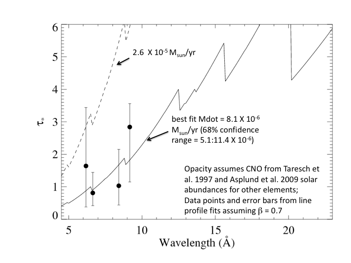
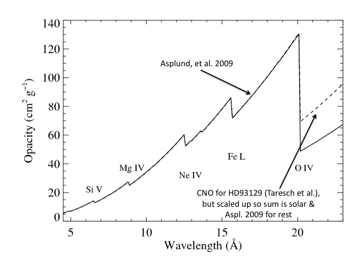
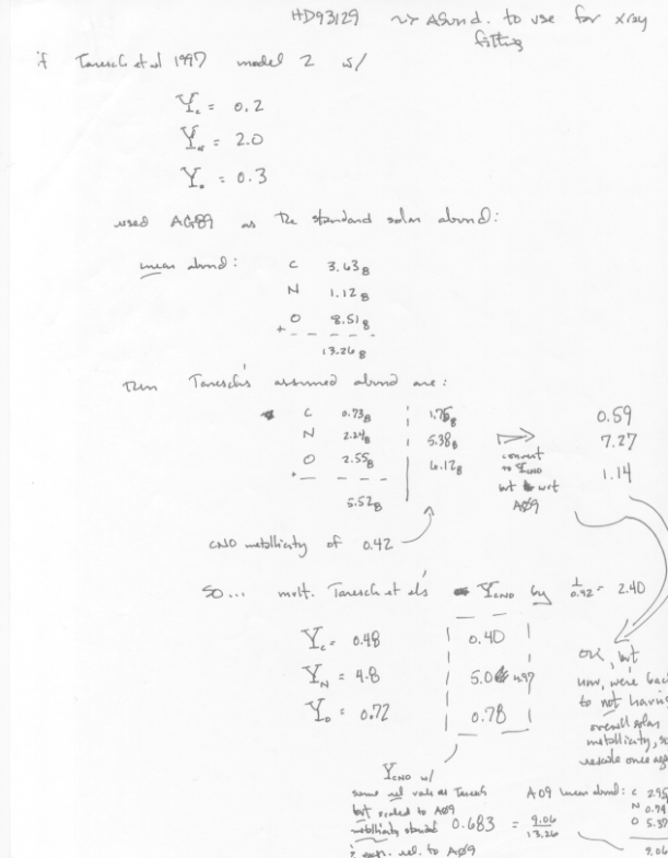
Using a model of the wavelength-dependent opacity, we can derive a mass-loss rate by fitting the set of taustar values derived above. For the two different models of wind opacity (solar/Asplund2009 and CNO-subsolar/Taresch1997), and using the β = 0.7 fits from above, we have the following determinations:

Solar

Altered CNO

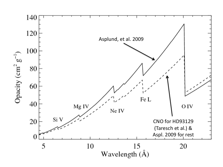
Here is a plot of the two different opacity models. Note that the sum of C, N, and O in the altered model is only 68% solar.

New:
Altered CNO, but sum rescaled to solar

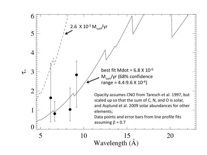
Note that the result here - the mass-loss rate of 6.8 X 10^-6 - is the same as for the solar abundance opacity model. The altered CNO (once their sum is rescaled to solar metallicity) only affects the opacity longward of the O K-shell edge, and there are no lines in the HD 93129A spectrum at those long wavelengths. Here is a plot of the opacity model, compared to the standard solar abundance opacity model.

New:
including the fifth line, S XV

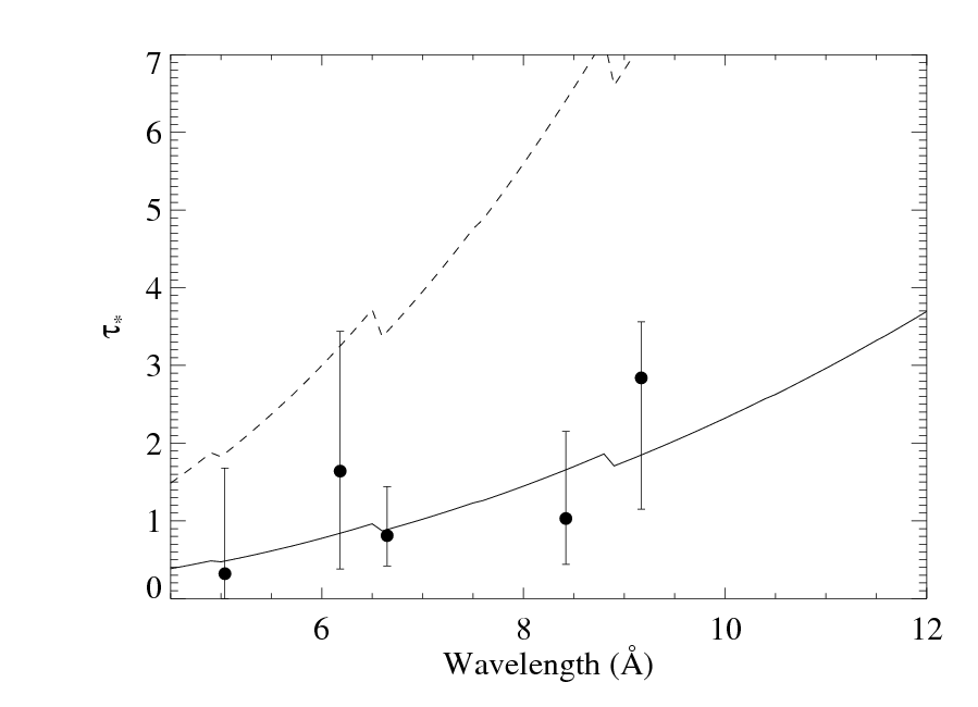
The result is unchanged: The mass-loss rate is 6.8 X 10^-6 Msun/yr.

R_o determination

The plot below summarizes the onset radii, R_o, determined from the line profile fits, above, using β = 0.7.

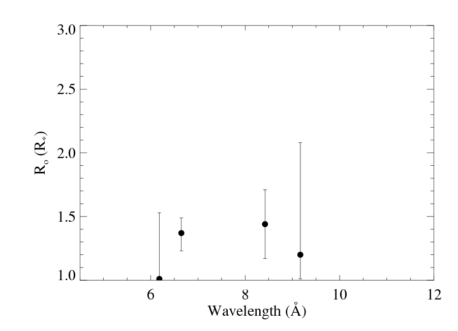
New: with a fifth line, S XV, included.

Overall summary of line profile fits

Finally, here is a text summary of the important parameter fits for both cases of β.

 

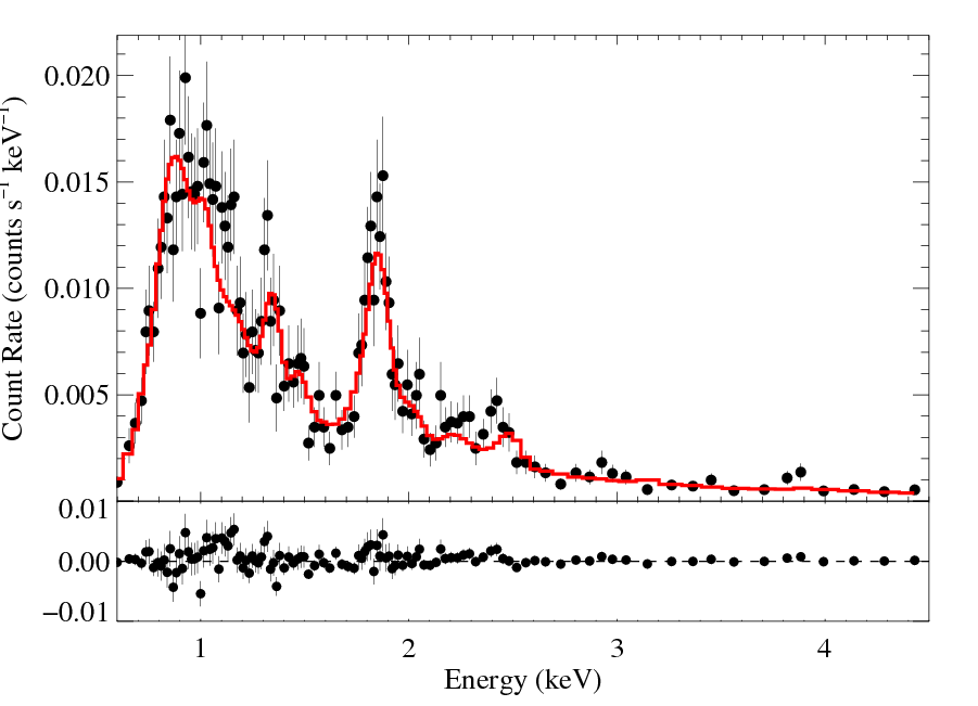
Global (VAPEC * windtabs) thermal spectral modeling

Here we fit the zeroth-order ACIS CCD spectrum with a multi-temperature APEC model, allowing for variable abundances (VAPEC), in conjunction with a broadband wind attenuation model (windtabs) for the cooler of the two temperature components. The model includes ISM attenuation (of both emission components) via tbabs. We allow the ISM column density to be a free parameter, and find values very consistent with that derived from the observed reddening (NH = 3.7e21).

MEG	[0.5:5.0], keV T1 = 0.61 keV   +/- (0.59:0.63) norm1 = 3.13e-3   +/- (2.85e-3:3.77e-3) T2 = 3.31 keV   +/- (2.32:5.42) norm2 = 1.72e-4   +/- (1.11e-4:2.24e-4) Σ* = 0.0522 g/cm2   +/- (0.0376:0.0707) NH = 4.1e21 cm-2   +/- (3.5e21:5.0e21) rejection probability = 40% (ChiSq = 114.86; N=118)

The mass column (Σ_*) implies a mass-loss rate of M-dot = 5.18 X 10^-6 Msun/yr (3.73e-6:7.01e-6). This is in very good agreement with the independent determination from the individual line profiles.

The abundances used in both the windtabs model and the vapec model assume solar after Asplund et al. (2009), but with C, N, and O altered, according to the ratio found by Taresh et al. Rescaled to the Asplund standard, these correspond to C:N:O = 0.25:3.02:0.47. Detailed notes on the rescaling can be found here: [1, 2, 3].

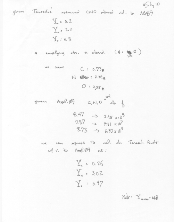
The flux from our best-fit model (corrected for ISM attenuation) is f_X = 6.60e-13, corresponding to L_X = 7.29e32 ergs/s (at d = 2300 pc). If we zero out the wind attenuation, we find that the intrinsic flux produced by our model corresponds to a luminosity of L_X = 3.30e33 ergs/s. This is the X-ray power requirement of any model that attempts to explain the X-ray production in this star. This wind-absorption-corrected spectrum is shown as a second histogram in this figure from the manuscript.

 

Back to the top

---

last modified: 31 January 2011