iota Ori: Chandra grating spectrum
There is a relatively short (49920 s) HETGS observation in the archive (looks like a GTO; it comprises two obs ids, which I've added together for the spectral analysis below). This object/data didn't make it into Emma's sample. Here, we take a quick look at it, prompted by Marc's noting that its lines are very broad.
This star is in Erin's sample, though not in the supergiant subsample that she focused on. But she did do a literature search on its stellar and wind properties, the results of which are summarized in this table. It is listed as O9 III with a binary companion (it's actually a multiple star system, with several wide companions that Chandra could resolve if their X-ray fluxes were high enough, and a spectroscopic companion in a highly eccentric orbit). With a periastron of something like 0.1 AU, wind-wind X-rays are a possibility. But for most of the orbit, the separation probably precludes significant CWB X-rays.
The wind speed determined from UV lines is indeed rather high, but not overly so. We will adopt 2350 km/s from S. Haser's dissertation. The Munich group (Puls et al. 2006) uses 2300 km/s. The brightest star in Orion's sword, it is also known as HD 37043 and 44 Ori. Here are its Simbad entry and the Simbad reference summary, Encyclopedia of Science entry, an optical image of the field, speculation about previous gravitational interactions, Kaler's page, and of course iota Ori's Wikipedia page.
The O Star Catalog (Maiz-Apellaniz et al. 2004) entry:


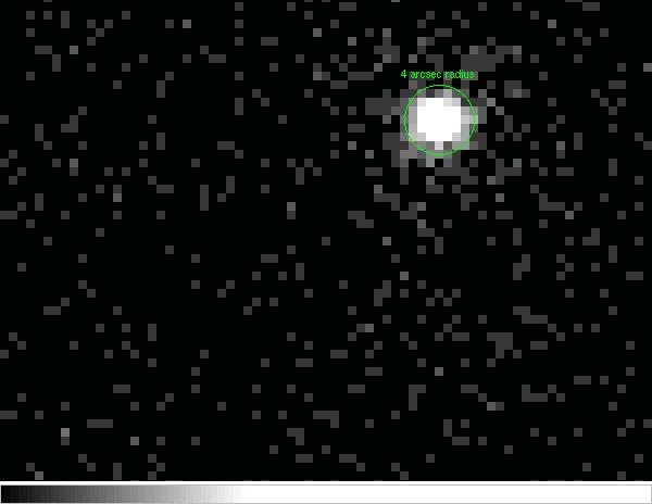
TGCAT says that the field is crowded, but there appear to be no sources very close to iota Ori, as can be seen in this image of the center of the ACIS detector. Zooming in, we can see that the zeroth order spectrum is well centroided. For each of the two Obs IDs, we re-reduced the data, starting with the level 1 events table, and produced a new pha2 file as well as grating arfs and rmfs. We then added the two pha files together (and the garfs, too).
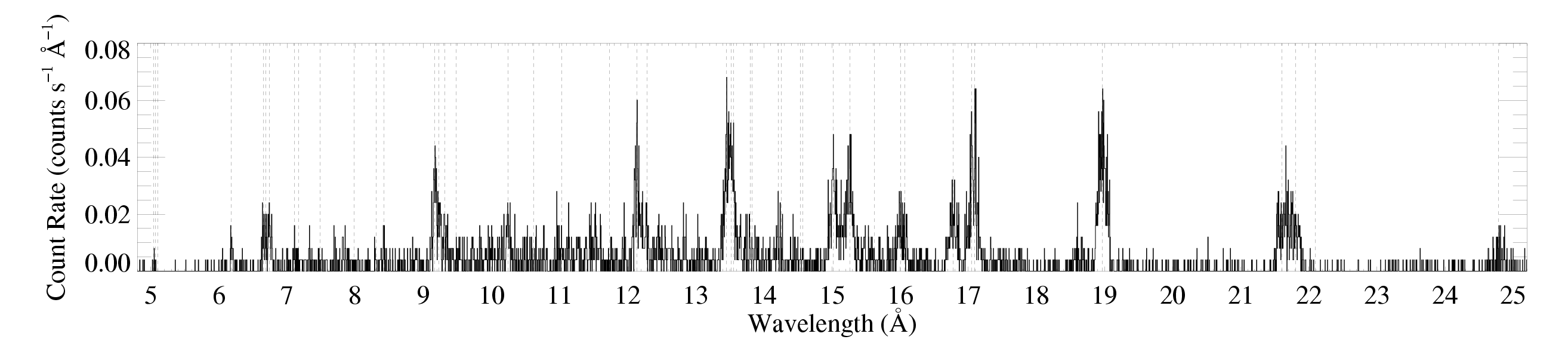
The HETGS spectra
MEG
HEG
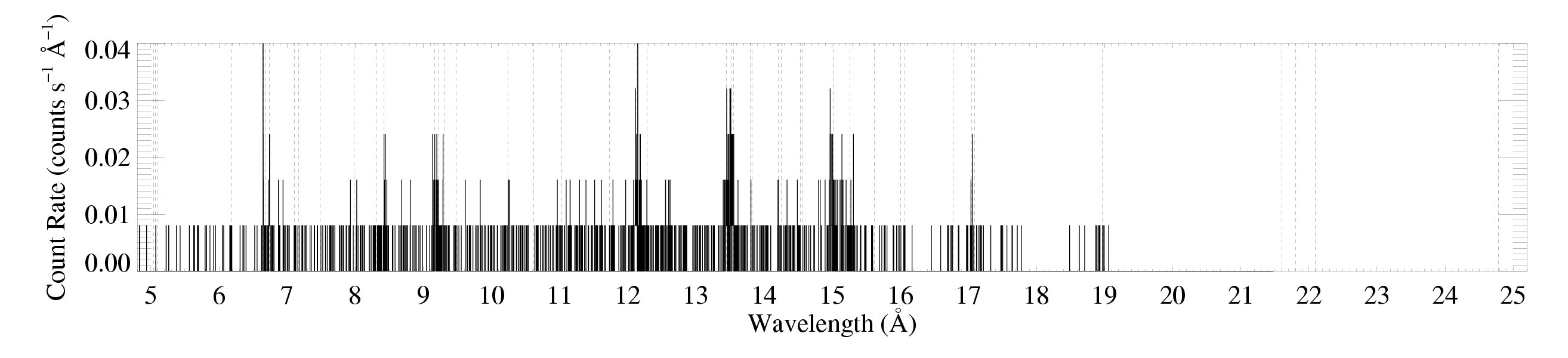
Note that there are very few HEG counts. In general, we will fit lines using only the MEG data.
The profile fitting shown below was done in xspec with the windprofile custom model.
The work shown below - fitting of individual lines - now (as of 6Aug09) includes both Obs IDs
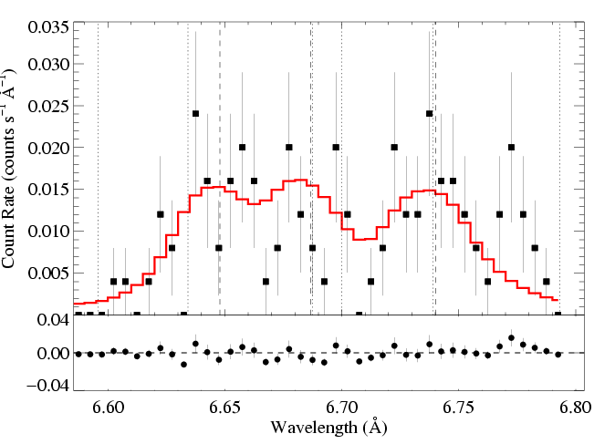
6.6479, 6.6866, 6.7403 Angstroms: Si XIII
MEG
HEG 
|
[6.58:6.80], λo = 6.6479, 6.6866, 6.7403
vinf=2350 β=1 powerlaw continuum, n=2; norm=1.24e-4 q=0 hinf=0 taustar=0.09 +/- (0.00:0.30) 0.00:0.53 at 90% confidence Ro=1.38 +/- (1.29:1.55) G=1.93 +/- (1.53:2.46) norm=1.47e-5 +/- (1.35e-5:1.64e-5) rejection probability = ???% (C=204.12; N=260) fit log |
Here are the 68%, 90%, and 95% joint confidence limits on taustar and Ro. The filled circle represents the best-fit model, shown as the red histograms on the above plots.
|
Note the very high G value. Probably this is due to (unaccounted for) blending with Mg Ly-beta. The S/N of this complex is quite low; modeling the blend will probably introduce systematic errors. We probably should exclude this complex from our analysis.
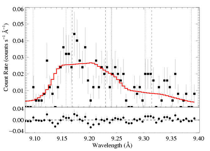
9.1687, 9.2297, 9.3143 Angstroms: Mg XI
MEG
HEG 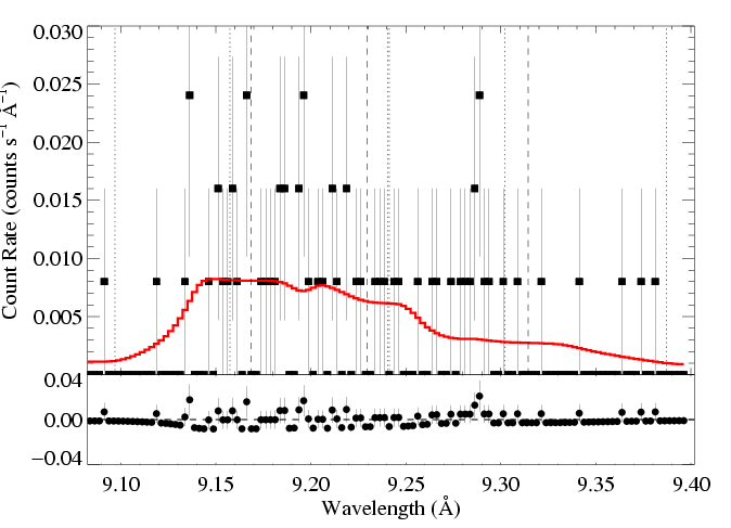
|
[9.08:9.40], λo = 9.1687, 9.2297, 9.3143
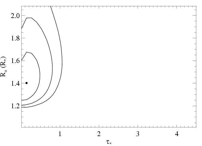
vinf=2350 β=1 powerlaw continuum, n=2; norm=4.12e-4 q=0 hinf=0 taustar=0.10 +/- (0.00:0.38) 0.00:0.65 at 90% confidence Ro=1.64 +/- (1.52:1.88) G=1.07 +/- (0.89:1.31) norm=3.29e-5 +/- (3.08e-5:3.61e-5) rejection probability = ???% (C=343.80; N=380) fit log |
Here are the 68%, 90%, and 95% joint confidence limits on taustar and Ro. The filled circle represents the best-fit model, shown as the red histograms on the above plots.

|
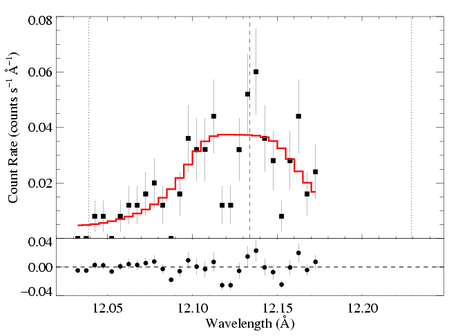
12.134 Angstroms: Ne X Ly-alpha
MEG
HEG 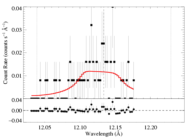
|
[12.03:12.18], λo = 12.134
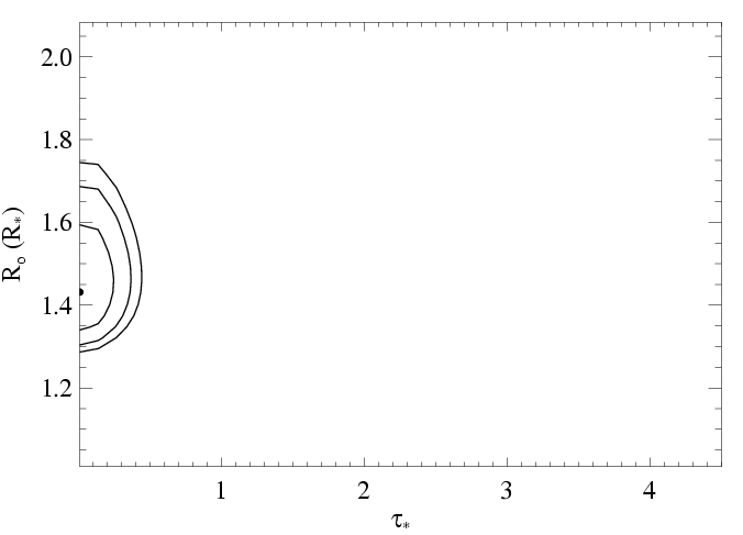
vinf=2350 β=1 powerlaw continuum, n=2; norm=1.29e-3 q=0 hinf=0 taustar=0.00 +/- (0.00:0.17) 0.27 at 90% confidence Ro=1.44 +/- (1.37:1.54) norm=6.62e-5 +/- (6.1e-5:7.2e-5) rejection probability = 89.8% (C=180.41; N=176) fit log |
Here are the 68%, 90%, and 95% joint confidence limits on taustar and Ro. The filled circle represents the best-fit model, shown as the red histograms on the above plots.
|
Note that the fit quality is not that good. Looking at the MEG data, there does appear to be some weird structure or scatter in the data. It's doubtful that any smooth model could provide a good fit to these data. I saw the same basic behavior when I fit only one Obs ID.
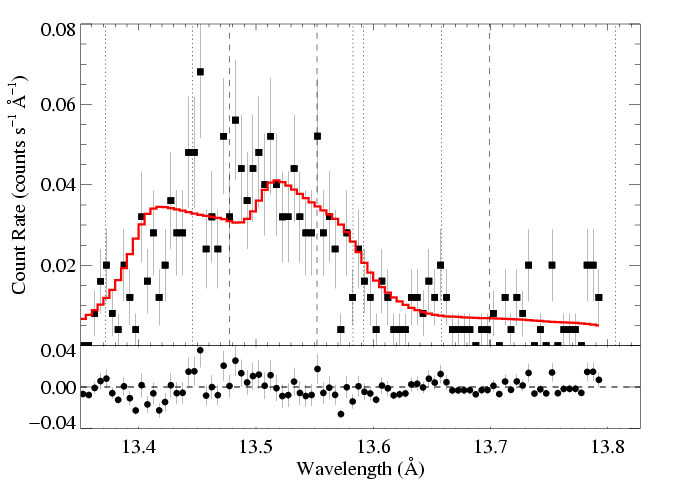
13.447, 13.552, 13.699 Angstroms: Ne IX
MEG
HEG 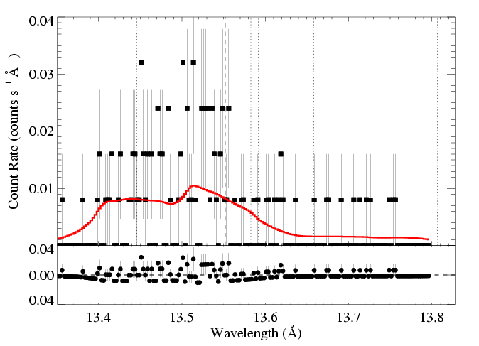
|
[13.34:13.80], λo = 13.4473, 13.5523, 13.6990
vinf=2350 β=1 powerlaw continuum, n=2; norm=2.15e-3 q=0 hinf=0 taustar=0.24 +/- (0.07:0.50) 0.00:0.69 at 90% confidence Ro=1.68 +/- (1.61:1.79) G=1.21 +/- (1.04:1.43) norm=2.53e-4 +/- (2.39e-4:2.67e-4) rejection probability = ???% (C=512.78; N=548) fit log |
Here are the 68%, 90%, and 95% joint confidence limits on taustar and Ro. The filled circle represents the best-fit model, shown as the red histograms on the above plots.
|
Note that this is the only line (complex) for which taustar.ne.0. It could be affected by blending with Fe lines. (update: this was before I fit the Mg XI complex, which also has a non-zero best-fit taustar.)
15.014 Angstroms: Fe XVII
MEG

HEG 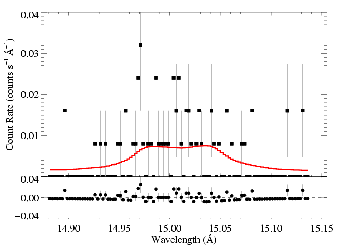
|
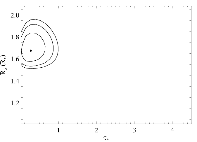
[14.88:15.14], λo = 15.014
vinf=2350 β=1 powerlaw continuum, n=2; norm=5.17e-3 q=0 hinf=0 taustar=0.00 +/- (0.00:0.03) 0.10 at 90% confidence Ro=1.56 +/- (1.47:1.78) norm=1.64e-4 +/- (1.48e-4:1.85e-4) rejection probability = ???% (C=129.70; N=102) fit log |
Here are the 68%, 90%, and 95% joint confidence limits on taustar and Ro. The filled circle represents the best-fit model, shown as the red histograms on the above plots.
|
Zoom in on the allowed region.
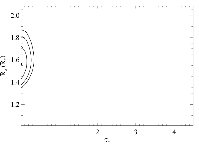
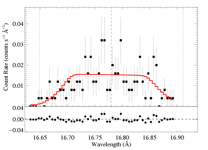
16.780 Angstroms: Fe XVII
MEG
|
[16.63:16.90], λo = 16.780
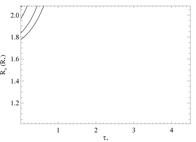
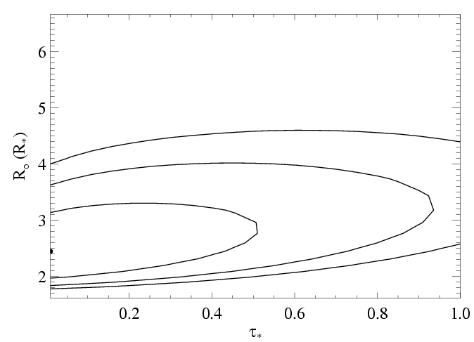
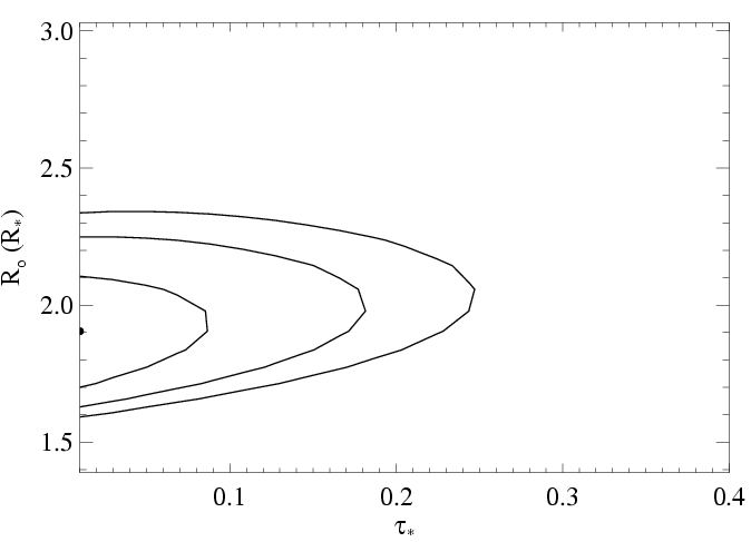
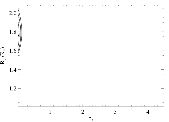
vinf=2350 β=1 powerlaw continuum, n=2; norm=6.42e-4 q=0 hinf=0 taustar=0.00 +/- (0.00:0.27) 0.58 at 90% confidence Ro=2.35 +/- (2.09:2.93) norm=1.82e-4 +/- (1.66e-4:1.98e-4) rejection probability = ??% (C=122.69; N=106) fit log |
Here are the 68%, 90%, and 95% joint confidence limits on taustar and Ro. Note that the best-fit model is off the top of this plot, on the standard axis ranges we use.
|
Zoom in and recenter on the allowed region.
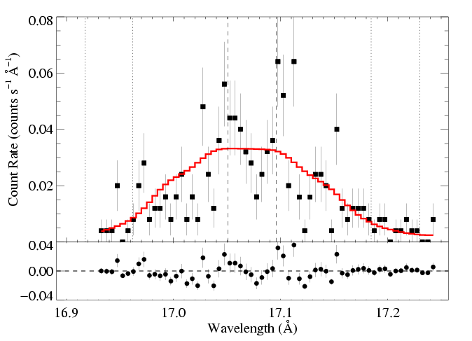
17.051, 17.096 Angstroms: Fe XVII
MEG
|
[16.93:17.25], λo = 17.051, 17.096
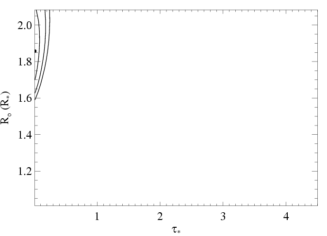
vinf=2350 β=1 powerlaw continuum, n=2; norm=2.21e-3 q=0 hinf=0 taustar=0.00 +/- (0.00:0.04) 0.10 at 90% confidence Ro=1.85 +/- (1.74:2.02) norm=1.90e-4, 1.71e-4 +/- (1.78e-4:2.03e-4) rejection probability = ??% (C=167.97; N=126) fit log |
Here are the 68%, 90%, and 95% joint confidence limits on taustar and Ro. The filled circle represents the best-fit model, shown as the red histograms on the above plot.
|
Zoom in on the allowed region.
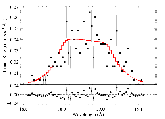
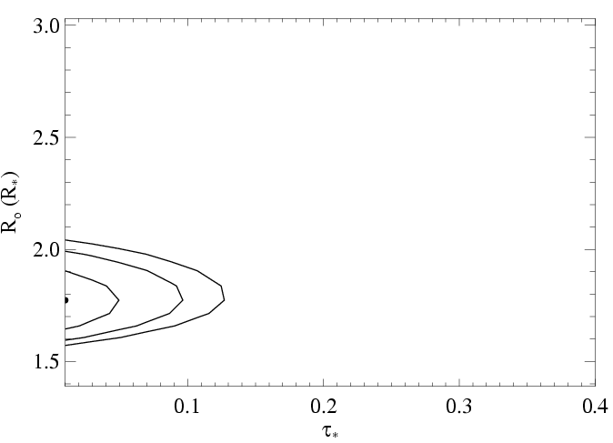
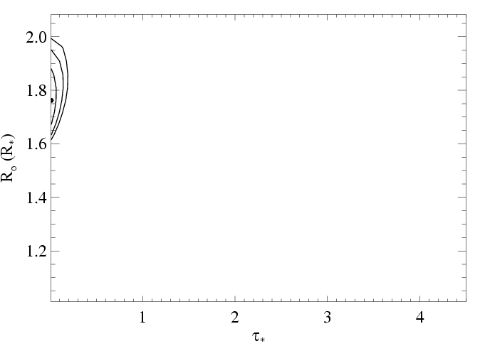
18.969 Angstroms: O VIII Ly-alpha
MEG
|
[18.81:19.12], λo = 18.969
vinf=2350 β=1 powerlaw continuum, n=2; norm=2.64e-3 q=0 hinf=0 taustar=0.00 +/- (0.00:0.02) 0.06 at 90% confidence Ro=1.75 +/- (1.67:1.86) norm=8.64e-4 +/- (8.18e-4:9.18e-4) rejection probability = ??% (C=145.74; N=122) fit log |
Here are the 68%, 90%, and 95% joint confidence limits on taustar and Ro. The filled circle represents the best-fit model, shown as the red histograms on the above plot.
|
Zoom in on the allowed region.
21.602, 21.804, 22.097 Angstroms: O VII
MEG

|
[21.4:22.1], λo = 21.602, 21.804, 22.097
vinf=2350 β=1 powerlaw continuum, n=2; norm=1.03e-3 q=0 hinf=0 taustar=0.00 +/- (0.00:0.03) 0.08 at 90% confidence Ro=1.76 +/- (1.69:1.84) G=0.96 +/- (0.85:1.11) norm=1.55e-3 +/- (1.47e-3:1.65e-3) rejection probability = ??% (C=236.97; N=278) fit log |
Here are the 68%, 90%, and 95% joint confidence limits on taustar and Ro. The filled circle represents the best-fit model, shown as the red histograms on the above plot.
|
last modified: 25 August 2009