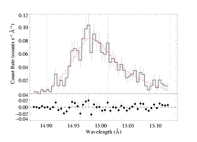
Fe XVII 15.014 Angstroms
Models with anisotropic porosity - clumps shaped like pancakes
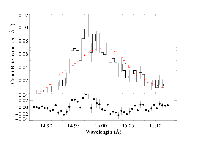
As in the case with the isotropic porosity models - when we use an anisotropic model of porosity (pancake-shaped blobs), we find that a porosity length of zero is preferred. So, the best-fit model shown below looks, and is, basically identical to the non-porous best-fit model and to the isoporous best-fit model. Note that this model sets the "rosseland" parameter to zero; in other words, it uses the exponential bridging law.
|
[14.87:15.13]
vinf=2250 β=1 powerlaw continuum, n=2; norm=1.91e-3 q=0 hinf=0.00 +/- (0.00:0.27) and for 90% confidence, (0.00:0.49) taustar=1.95 +/- (1.67:2.35) uo=0.651 +/- (0.605:0.727) norm=5.27e-4 +/- (5.04e-4:5.50e-4) rejection probability = 21% (C=95.10; N=102) |
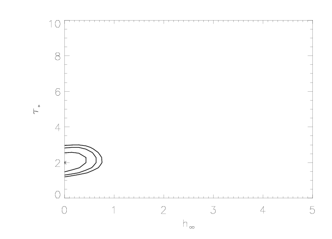
Note that the upper limit on taustar is better constrained than for the isoporous case. This is a sign that anisotropic porosity models provide worse fits to the data than isotropic porosity models. This can be seen below, where we show the joint confidence limit plots, and the confidence limits on hinf are quite constrained.

Note here that because anisotropic porosity leads to line profiles that don't look like the data, not only are significant values of hinf ruled out, but these second set of confidence limits (taustar vs uo) look nearly identical to those from the non-porous model fits (i.e. playing with anisotropic porosity does not help improve the quality of the model fits for any combination of taustar and uo).
New: We also fit the anisotropic porosity model to the combined MEG and HEG data, and got similar results - best-fit is no porosity; fit gets bad very quickly as the porosity length increases. The constraints are even tighter: 68% upper limit on hinf is just 0.06 and 90% is 0.17. For the record, here are the parameters of the anisoporous fit (these aren't quite the best-fit parameter values, but we wanted to show which switches/options we used). We do not show the best-fit model on the two datasets here because the models are nearly indistinguishable from the one we show at the top of this page, fit only to the MEG data. But the confidence limits should be affected by the inclusion of the additional data in the fits.
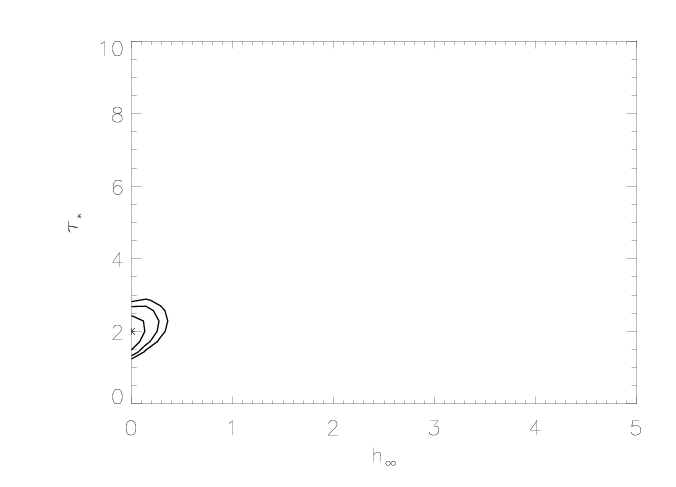
Here are the joint confidence limits on hinf and taustar from the combined fit to the MEG and HEG data:
And here are the joint confidence limits on taustar and uo from the combined fit to the MEG and HEG data:
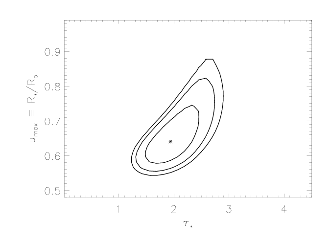
Note that as with the isoporous models, the inclusion of the HEG data in the fits constrains uo enough to rule out plasma right at the photosphere (even, presumably, for models with very large porosity lengths). The relative constraints are even tighter in this case, probably because anisoporous models are bad overall.
As we do for the isotropic porosity modeling, we investigate the extent to which porosity can explain the profile shape in the context of higher mass-loss rates. Specifically, if the literature mass-loss rate is correct, then (a) can porosity explain the relatively symmetric profile (as well as a reduction in mass-loss rate in the context of a non-porous wind can) and (b) what levels of porosity (what values of hinf) are required?
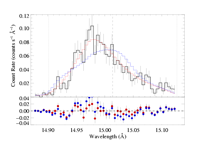
The best-fit model with anisotropic porosity and taustar fixed at 8:
|
[14.87:15.13]
vinf=2250 β=1 powerlaw continuum, n=2; norm=1.91e-3 q=0 hinf=2.92 +/- (2.28:3.65) and for 90% confidence, (1.97:4.31) taustar=8 uo=0.661 +/- (0.617:0.718) norm=5.27e-4 +/- (5.04e-4:5.50e-4) rejection probability = 96% (C=135.30; N=102) |
This fit is not good (unlike the high taustar fit with isotropic porosity, which isn't too bad). And of course, even if we accept this fit, it requires a very high value of hinf, as in the case of the isotropic porosity fit.
Here are the two models overplotted with the data: the red model is the global best fit, with taustar=2.0 and hinf=0.0, while the blue model is the best-fit in which taustar is held fixed at a value consistent with the literature mass-loss rate, taustar=8, and the best-fit value of hinf=2.92.
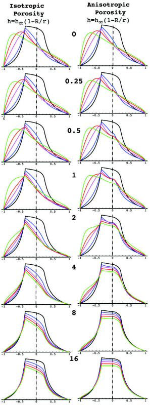
The poor fit is due to the fact that anisotropic porosity tends to cause and excess of emission near line center (this is the so-called "Venetian blind effect" - photons from the sides of the wind, where material is moving more or less across our line of sight and where the pancake-shaped clumps are oriented edge on, which enhances the escape probability). The anisotropic porosity models - to some extent like the isotropic porosity models - also show an emission excess on the extreme blue wing of the profile. These trends can be seen more clearly below, where we show the two models at high (infinite) resolution. The global nature of the trend in these features can also be seen in the suite of model comparisons.
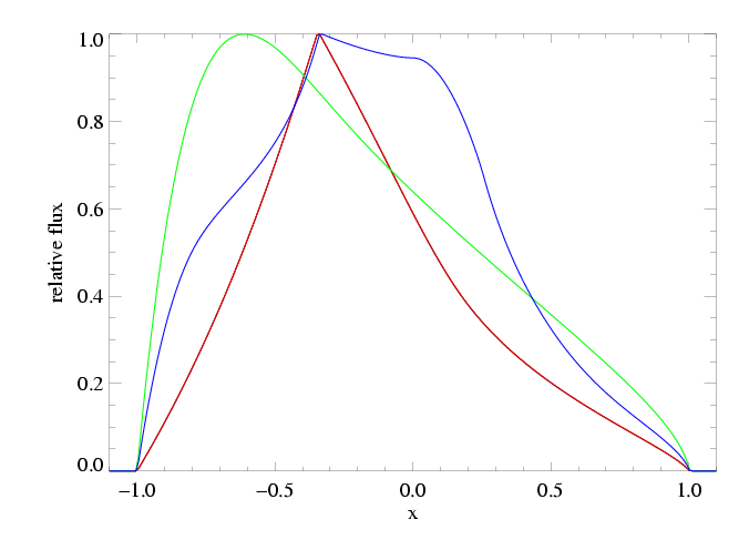
Here the best-fit global model (with hinf=0) is shown in red, the best-fit model with taustar=8 and anisotropic porosity is shown in blue, and the taustar=8 model with no porosity is shown in green. Note that the red and green models are identical to those shown in the plot at the bottom of the page on the isotropic porosity fit to this same line.
See how the inclusion of the the HEG data in the constrained (taustar=8, frozen) fit changes these results.
See how using the Rosseland opacity bridging law in the constrained (taustar=8, frozen) fit changes these results.
Back to main page.
last modified: 27 April 2008