σ Ori E: x-ray flux levels and spectral properties
The RFHD model
We will attempt to constrain the RFHD model, shown above, with broadband, low resolution x-ray data.
We begin by looking at the Chandra ACIS dataset (first published in Skinner et al. 2008) and the XMM EPIC dataset (first published in Sanz-Forcada et al. 2004). These instruments are both CCD arrays with energy response above about 0.5 keV and low spectral resolution. Much of the spectral shape visible in the datasets is a function of the instruments' energy-dependent effective area and resolution. Every indication is that the underlying spectra consist of optically thin thermal line emission with a relatively weak bremsstrahlung continuum.
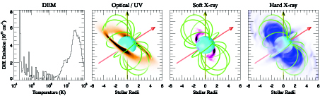
Our goals are to characterize the temperature distribution and x-ray luminosity of the thermal plasma emitting these x-rays, and to compare these quantities to the predictions of the RFHD modeling (Fig. 12 in Townsend, Owocki, & ud-Doula 2007). In addition to the time-averaged emission properties, there are also several issues of time variability involved: (i) Flares: the RFHD model itself does not model flares (related: can we ascertain which portions of the available x-ray data represent true quiescence?) (ii) How much short term variability is seen in the data during quiescence? Is it periodic? Rotationally modulated? (iii) Are there longer-term, secular changes in the quiescent emission levels?
Published data
There's ROSAT data in the archive and also a second Chandra dataset (taken with the HRC), which we will not discuss here (at least for now). The two datasets we will discuss are the XMM EPIC data and the Chandra ACIS data. Here is the EPIC light curve from Sanz-Forcada et al. 2004:
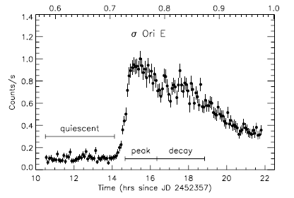
You can read the caption. Note the big flare. We'll focus, at first, on the quiescent portion of the observation.
Here are the EPIC spectra from the quiescent and peak portions:

Clearly, the spectrum gets substantially harder during the peak of the flare.
Here's the Chandra ACIS light curve from Skinner et al. 2008:
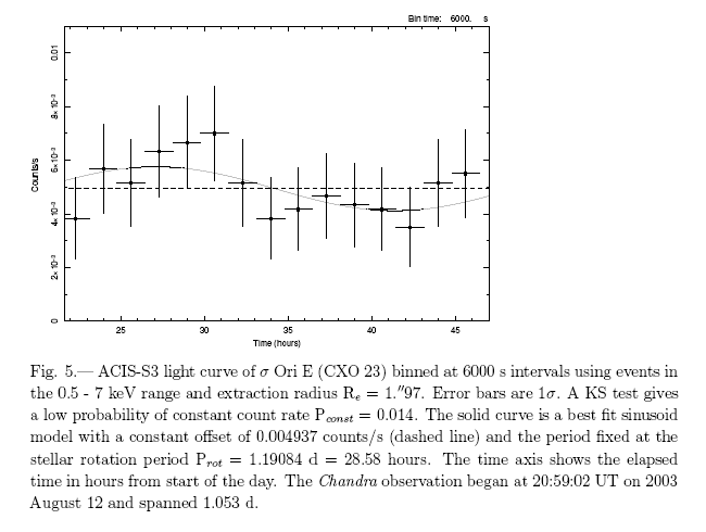
Clearly there was no flare during this observation, but there's mild evidence for rotational modulation, perhaps.
Here's the ACIS spectrum with a three-temperature thermal emission model fit to it:

One question we'll address below is whether this spectrum - both in terms of overall flux level and in terms of spectral energy distribution - is consistent with the quiescent XMM EPIC spectrum.
We will now reanalyze these data to answer some of the questions listed under goals near the top of the page.
The Chandra ACIS data
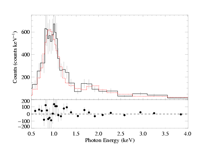
Here is the best-fit 2-temperature APEC model:
|
NISM = 3 X 1020 cm-2 T1 = 0.73 +/- 0.60:0.81 keV EM1 = 6.2 X 1052 +/- 5.0:7.9 X 1052 cm-3 T2 = 2.42 +/- 1.88:3.17 keV EM2 = 1.5 X 1053 +/- 1.1:1.7 X 1053 cm-3 rejection probability = 74% (Χ2 = 31.3; N = 31, so Χ2ν = 1.16) |
Notes: Parameters without uncertainties listed were held frozen during the fitting (here, the ISM column density was fixed). The quoted uncertainties are actually lower and upper 90% confidence limits. The rejection probability is based on the reduced chi square (Χ2ν) value and the number of degrees of freedom (number of data points, N - # of free model parameters). The emission measures are calculated from the component normalizations assuming a distance of 352 pc. Elemental abundances are assumed to be solar.
The above 2-T APEC fit is adequate. However, the assumption of two discrete temperatures is not physically realistic, so we next fit a continuous temperature distribution (a differential emission measure, or DEM, model).
We use the XSPEC model c6pmekl, which describes the DEM using a 6th order Chebyshev polynomial. The underlying model is the MeKaL thermal emission model, which makes the same assumptions as the APEC model (different compilation of atomic data and ionization balance, though).
Here is the best-fit c6pmekl model:
|
NISM = 3 X 1020 cm-2 normalization = 3.5 X 10⁻⁶ rejection probability = 60% (Χ2 = 25.1; N = 31, so Χ2ν = 1.05) |
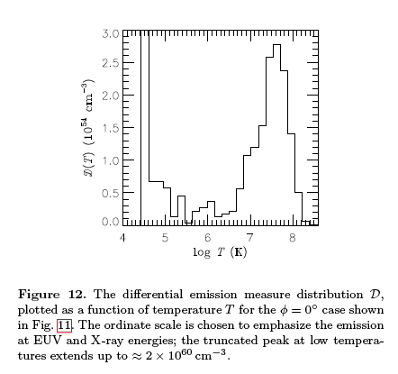
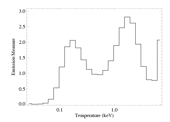
It's not immediately obvious how to compare the quality of this fit to that of the 2-T fit. Χ2 improved, but there are fewer degrees of freedom. The rejection probability is lower, though, so in that sense the fit is clearly an improvement. We don't list the six Chebyshev coefficients because they're hard to interpret, physically. But instead, we show a graphical description of the DEM below:
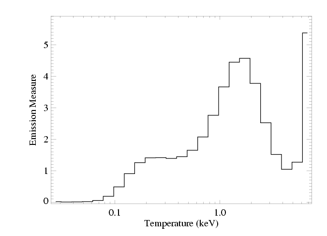
Semi-quantitatively, this DEM looks like the theoretical DEM from the RFHD simulations. The peak temperature of the DEM derived from the data is at a slightly lower temperature than that predicted by the model. Note: The rising DEM at very high temperatures is almost certainly spurious. Functionally, it's contributing bremsstrahlung continuum to the model spectrum (and not lines), so it's likely that the DEM model doesn't provide a strong enough continuum and the fitting routine is compensating by adding a very hot component to provide the missing continuum. If, indeed, the continuum in the model is too weak, it's most likely due to sub-solar abundances, which we haven't modeled (because determining abundances from low-resolution X-ray data is not reliable).
The flux of the best-fit c6pmekl model is 2.39 X 10⁻¹³ erg cm-2 s-1.
The XMM EPIC data
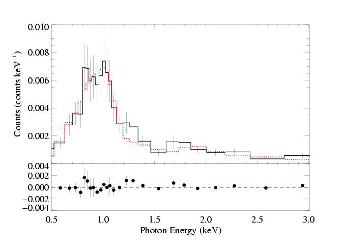
We first look at the EPIC spectrum formed from just the quiescent portion of the data. We show it here with the best-fit DEM (c6pmekl) model from the ACIS fitting shown above superimposed on it:

|
NISM = 3 X 1020 cm-2 normalization = 3.5 X 10⁻⁶ rejection probability = 100% (Χ2 = 694.5; N = 17, so Χ2ν = 77.2) |
OK - the quiescent XMM EPIC data clearly has a lower x-ray flux than the Chandra ACIS data. (Note that the x-axis range is the same for both these plots, but the y-axis range is different - and not comparable, since they're both in counts units and these units depend not just on the intrinsic flux but also on the energy-dependent effective areas of the two instruments. There are negligible counts at energies above the last bin shown.) It looks like the EPIC data implies a flux that's 2 to 3 times lower, but spectrally quite similar. We will quantify this next.
Renormalizing the c6pmekl model, we find:
|
NISM = 3 X 1020 cm-2 normalization = 1.4 X 10⁻⁶ rejection probability = 62% (Χ2 = 17.1; N = 17, so Χ2ν = 1.07) |
The flux of this renormalized c6pmekl model is 9.53 X 10⁻¹⁴ erg cm-2 s-1.
Note though, that since we kept the 6 coefficients frozen at their values derived from the fit to the ACIS data, they're not counted against our degrees of freedom. So, we're really saying the good fit (38% rejection probability) is true only given the DEM shape derived from fitting the ACIS data. If we take that as given, then the agreement is good. But that's reasonable, because we're asking the question, "are the EPIC data consistent with the ACIS data?" Note that if we assume we've only got 10 degrees of freedom (as if we'd let the 6 Chebyshev polynomial coefficients be free), then we've still got a rejection probability (92% for Χ2ν = 1.7 given ν = 10) that's not too bad. Clearly, we should also fit both datasets simultaneously, forcing the DEM shape to be the same but allowing for different normalizations. But first, let's state some tentative conclusions and then look at how the EPIC fit can be improved.
Tentative conclusions from fitting the two data sets separately: The normalization and thus the flux is 2.5 times lower for the EPIC, but even with exactly the same form of DEM that fit the ACIS data, we get a good fit to the EPIC data. In other words, both datasets are consistent with the same DEM model shape, though with normalizations that differ by a factor of 2.5.
Said another way, the purported temperature difference between the Chandra and XMM data that's reported in the literature (1.1 keV for the hot component of a multi-temperature - but not continuous DEM - model reported by Sanz-Forcada et al. for their fits to the EPIC data and the roughly twice as high temperature derived by Skinner et al. from the ACIS data) is not statistically significant. But the difference in the overall x-ray flux levels between the two observations is highly significant.
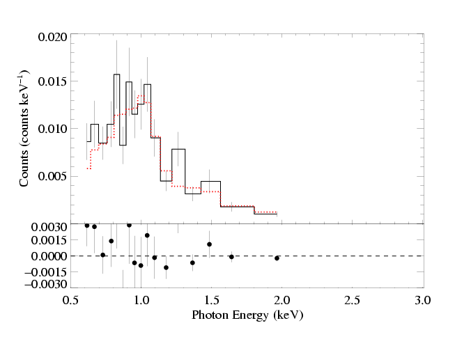
Now, although the DEM shape derived from the ACIS data provides an adequate fit to the EPIC data, it is surely not the best-fit. Below, we show the best-fit DEM, allowing all 6 Chebyshev coefficients to be free parameters, along with the normalization.
|
|
NISM = 3 X 1020 cm-2 normalization = 2.3 X 10⁻⁶ rejection probability = 82% (Χ2 = 13.9; N = 17, so Χ2ν = 1.39) |
Note that this fit isn't great (though it wouldn't even be excluded at the 90% level). Perhaps by varying the attenuation, the fit can be improved. But more importantly, the DEM shape from the ACIS best-fit model provides a fit that isn't much worse. The difference in chi square values between these two fits is Δχ2 = 3.2, which is not significant for a model with seven free parameters.
The flux of this best-fit c6pmekl model is 9.92 X 10⁻¹⁴ erg cm-2 s-1. This is 2.4 times less than that derived from the best-fit model to the ACIS data.
Here is the best-fit DEM:
compare it to the original best-fit ACIS DEM:
Interestingly, the peak of the EPIC best-fit DEM is no cooler than the model that provides the best fit to the ACIS data. But the cooler component is much stronger. I'm sure that many other DEM shapes would provide adequate fits to the data. After all, the ACIS best-fit DEM does.
last modified: 5 May 2008