ζ Pup: XMM RGS line-profile analysis
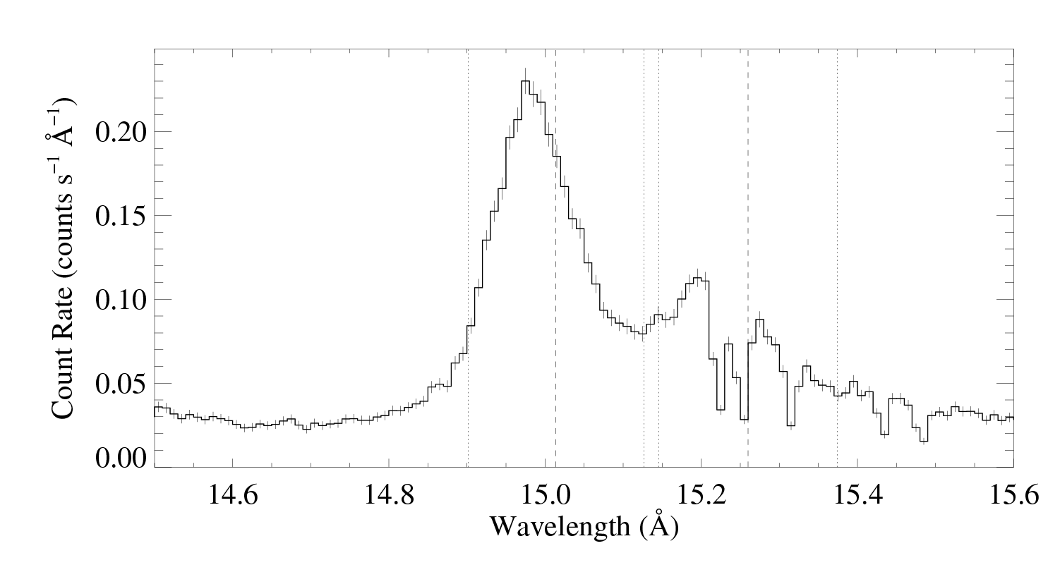
Initial tests on 15.014 Angstroms: Fe XVII
There is some blending on the red side of the line, with Fe XVII 15.26. (RGS1 on the left, and RGS2 on the right):

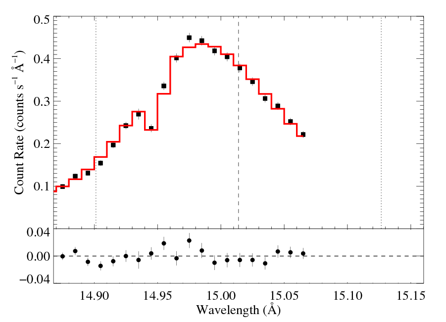
So, we fit the line on the wavelength interval 14.80 to 15.07 Angstroms. (We also fit the continuum at the same time as the line itself.) The results are shown below, where we co-add the RGS1 and RGS2 data and model for display purposes (the two spectra were fit as separate datasets, but fit jointly (i.e. simultaneously by the same model)). We use chi-square as the fit statistic, with Churazov error weighting. And we subtract the background from the data prior to fitting.

|
[14.80:15.07]
vinf=2250 β=1 powerlaw continuum, n=2; norm=3.23e-3 q=0 hinf=0 taustar=1.84 uo=0.636 norm=6.41e-4 rejection probability = xx (chisq=110.34; N=52) |
Note that this best-fit model is quite similar to the one we fit to the same line in the Chandra spectrum.
Note also that the reduced chi-square value of the fit is about 2.3, which is formally not a good fit. This is due to the very high signal-to-noise of the data. The formal error bars account only for statistical error, but these data are dominated by systematic (calibration) error. It's not clear how best to quantify the uncertainty (and, importantly, the confidence limits on the fitted model parameters). One approach would be to scale up the error bars to enforce a reduced chi square of unity for the best fit model -- thus effectively increasing the error bars by a factor of 2.3, and making corresponding changes to the confidence intervals). We have calculated delta-chi-square for a run of model parameter values. And without listing them here in detail, we'll note one example: the taustar estimate for the above fit ranges between 1.74 and 1.94 using naive 68% (delta-chi-square = 1) confidence limits. But if we scale the errors up by 2.3, then the 68% confidence range goes from 1.68 to 1.99 -- not a very big change.
Also note: because we were worried about contamination of the red wing of the line by the 15.26 line, we repeated the fit with only data shortward of 15.014 included, and we found a best-fit taustar = 2.00.
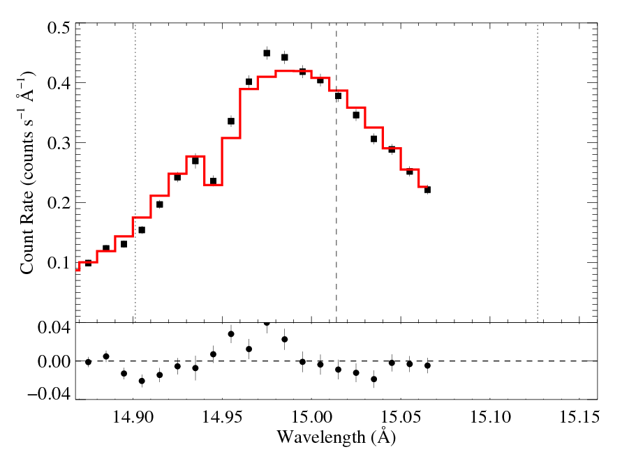
Next, we let the porosity length be a free parameter (the Rosseland bridging law was used), and hinf=0 was preferred, with the non-porous fit parameters recovered (i.e. the data do not favor porosity). Then, we fixed taustar at a value (taustar=5) corresponding roughly to the high, unclumped H-alpha mass-loss rate, froze taustar, and allowed the porosity length to be a free parameter, in order to explore the trade-off between taustar and hinf.
|
[14.80:15.07]
vinf=2250 β=1 powerlaw continuum, n=2; norm=3.07e-3 q=0 hinf=2.78 +/- (2.42:3.12) taustar=5 frozen uo=0.639 norm=6.42e-4 rejection probability = xx (chisq=125.07; N=52) |
So, delta chi square ~ 15; the non-porous model is strongly favored, though it's hard to quantify given the formally poor best-fit. If we scale by 2.3, then the delta chi square is only 6 (favoring the non-porous model at only the ~99% level).
Note that the quoted uncertainty on hinf also assumes the factor of 2.3.
We next refit the line, using a model with anisotropic porosity (Rosseland bridging law). We again find that porosity lengths of zero are preferred. And again fixing taustar at a high value, to represent the unclumped H-alpha rate, we fit the line, finding best-fit values of hinf and uo.
|
[14.80:15.07]
vinf=2250 β=1 powerlaw continuum, n=2; norm=2.71e-3 q=0 hinf=0.59 +/- (0.53:0.70) taustar=5 frozen uo=0.825 norm=6.58e-4 rejection probability = xx (chisq=192.96; N=52) |
This fit is significantly worse than the other two (delta chi square ~ 83 compared to the non-porous fit). It can even be seen to some extent in the data -- the model has something of a venetian blind effect that lies systematically above the data near line center.
Note also that uo is rather large, arguing against the applicability of the non-porous model.
last modified: 1 August 2011