ζ Pup: tradeoff between porosity and mass-loss rate reduction as constrained by line-profile data
Here we present our results from fitting individual lines with models without porosity ("non-porous"), isotropic porosity ("isoporous" - spherical clumps), and anisotropic porosity ("anisoporous" - flattened clumps). At the bottom of the page we summarize the results, looking at the mean values of key parameters as well as trends in these parameter values.
We examine in detail the key assumptions and parameter choices, as applied to one strong line on this page of background information. There we summarize preliminary conclusions and establish an analysis strategy, which we apply to the other line in the spectrum here.
Line-by-line results
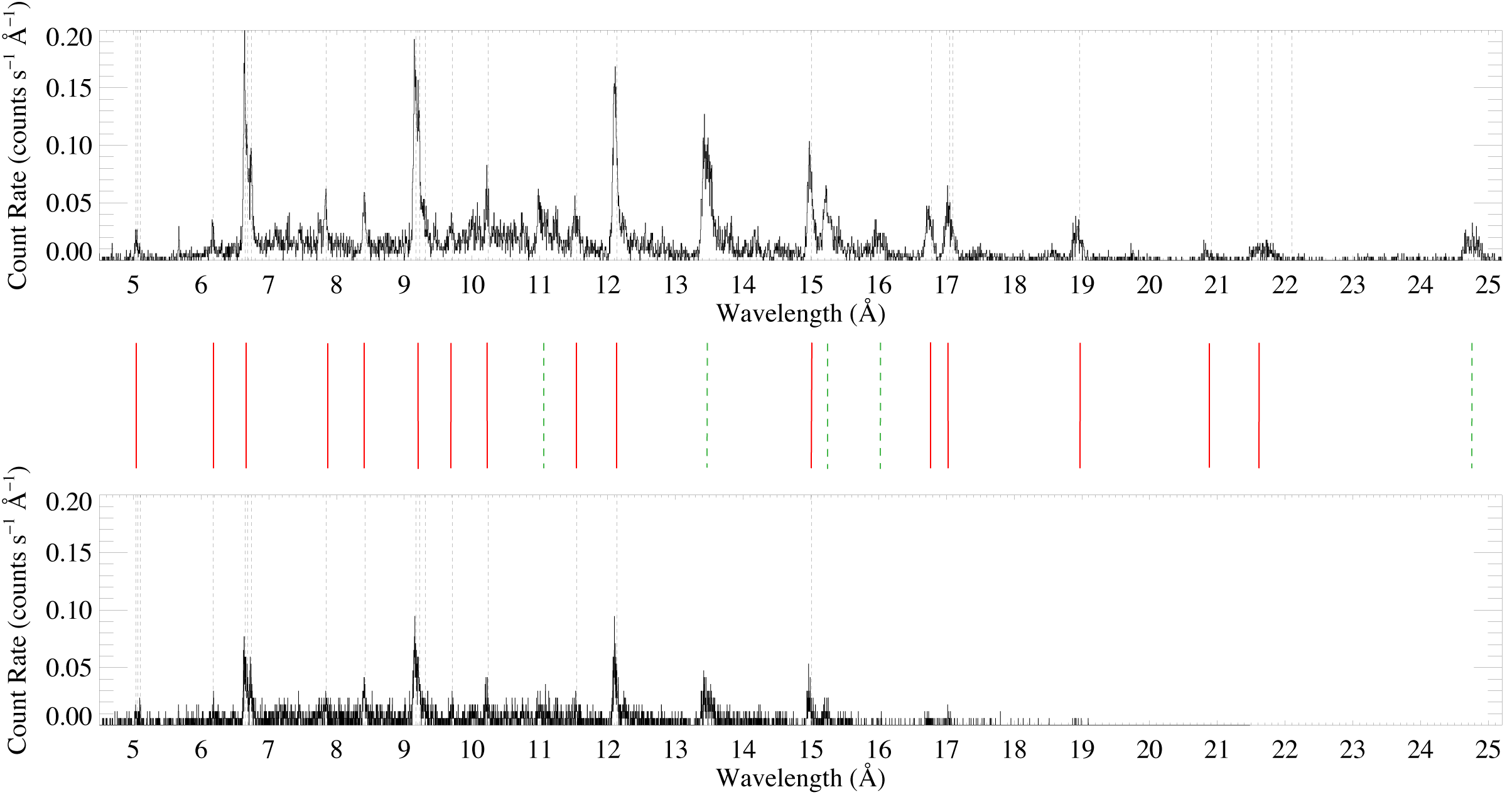
MEG

HEG
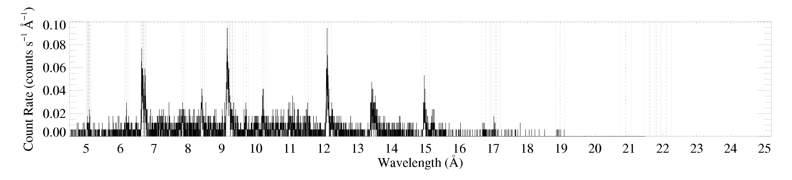
Note that the y-axis range is only half as big for the HEG plot. The vertical lines denoting the rest wavelength and the +/-vinf are shown only for the lines that we include in our analysis.
There is also an annotated plot updated to show the status of each line. Red indicates usable lines and dashed green indicates lines we attempted to fit but couldn't fit reliably because they're too blended.
5.039 Angstroms: S XV res., int., for. [non-porous]
6.182 Angstroms: Si XIV Ly-alpha [non-porous, isoporous, anisoporous]
6.648 Angstroms: Si XIII res., int., for. [non-porous]
7.850 Angstroms: Mg XI He-beta [non-porous]
8.421 Angstroms: Mg XII Ly-alpha [non-porous, isoporous, anisoporous]
9.1687 Angstroms: Mg XI res., int., for. [non-porous]
9.7082 Angstroms: Ne X Ly-gamma [non-porous]
10.239 Angstroms: Ne X Ly-beta [non-porous]
11.544 Angstroms: Ne IX He-beta [non-porous, isoporous, anisoporous]
12.134 Angstroms: Ne X Ly-alpha [non-porous, isoporous, anisoporous]
13.447 Angstroms: Ne IX res., int., for. [summary]
15.014 Angstroms: Fe XVII [non-porous, isoporous, anisoporous]
16.006 Angstroms: OVIII Ly-beta [summary]
16.780 Angstroms: Fe XVII [non-porous, isoporous, anisoporous]
17.051, 17.096 Angstroms: FeXVII [summary]
18.969 Angstroms: OVIII Ly-alpha [non-porous, isoporous, anisoporous]
20.910 Angstroms: N VII Ly-beta [non-porous]
21.602, 21.804 Angstroms: OVII res., int. [non-porous, isoporous, anisoporous]
24.781 Angstroms: NVII Ly-alpha [summary]
New: We have explored the nature of the confidence limits on two of the lines, showing several marginally well-fitting models, compared to the best-fit models.
Preliminary results: summary of non-porous fits
Note that these plots do not include results from the Ne IX complex near 13.5, the O Ly-beta line at 16.006, or the N Ly-alpha line at 24.781, because these lines/complexes are significantly blended with one or more other lines to the extent that their profiles cannot be reliably analyzed. That leaves 16 lines and line complexes that can be reliably fit with the wind profile model.
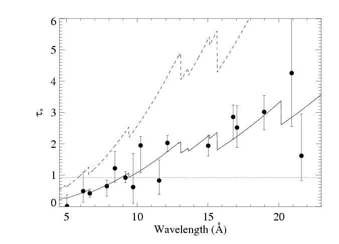
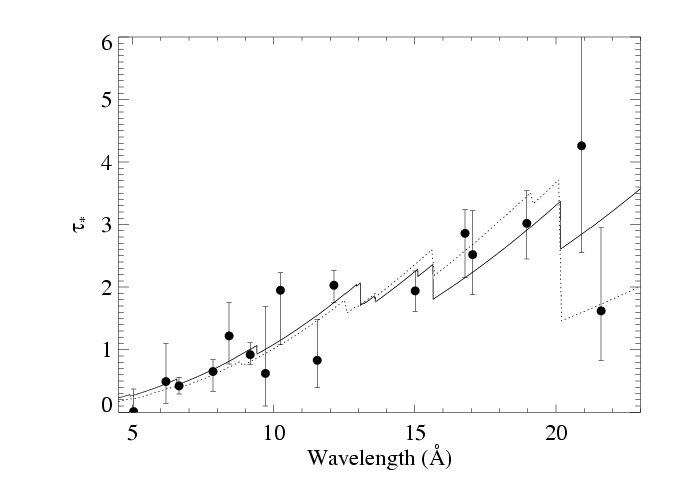
taustar

Note a modest trend in taustar with wavelength. This is qualitatively consistent with models of zeta Pup's wind opacity. This plot has important edges identified and the locations of important lines indicated.
We fit a model of taustar based on this opacity model, assuming a single M-dot value, and get a good fit with M-dot = 3.50 X 10⁻⁶ Msun/yr (solid curve, below) - with a 68 percent confidence interval of 3.25:3.73 X 10⁻⁶ Msun/yr. A constant taustar model (dash-dot line) cannot provide a good fit to the data (reduced chi square ~ 5.4 for 15 degrees of freedom). We show these two fits below, along with a model that uses the detailed wind opacity but forces M-dot = 8.3 X 10⁻⁶ Msun/yr (the dashed curve).
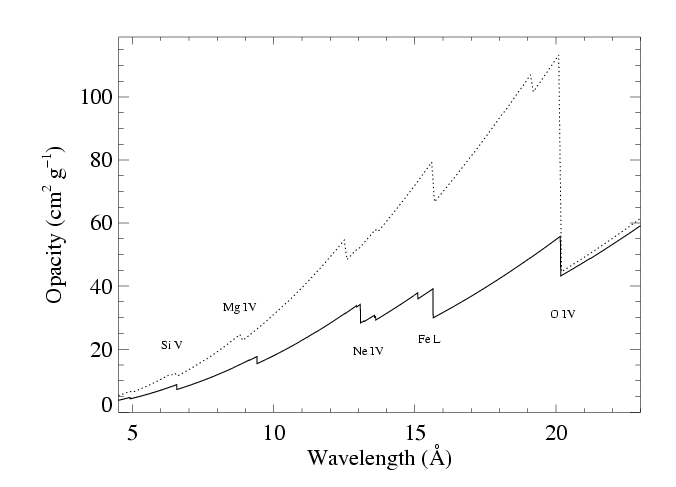
We have defined a "canonical" solar-abundance wind opacity model, which uses
Asplund, Grevesse, Sauval 2005 abundances for 30 elements (1 < Z < 30), cross sections from Verner & Yakovlev, and generic ionization balance for a nominal 40,000 K star, with values taken from MacFarlane, Cohen, and Wang 1994 for He, C, N, O, and Si, and +4 charge state assumed for every other element. We compare it to the cmfgen wind opacity model with abundances specific to ζ Pup, below (solid curve is cmfgen and dotted curve is solar).
And we refit the ensemble taustar values with a model parameterized by the mass-loss rate, using these opacities. We find a lower mass-loss rate, unsurprisingly, of 1.9e-6. The fit quality is about as good as for the N-enhanced cmfgen wind opacity model. The M-dot fit results are shown graphically, below. The solid curve is from the opacity model shown with the solid curve above, and is the same as in the figure above that. These models look almost the same, once their associated mass-loss rates are separately optimized.
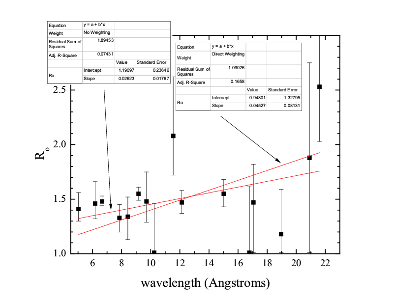
Ro
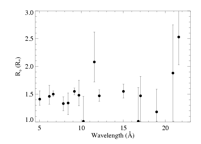
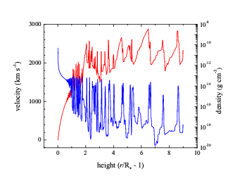
Note that most of the lines are consistent with the same onset radius of 1.4 to 1.5 Rstar. Some of the noisier lines are also consistent with locations much closer to the photosphere, but none require it. And the two highest signal-to-noise lines have significantly tighter constraints, with onset radii very close to 1.5 Rstar. This is completely consistent with the results of hydrodynamics simulations of the line-driven instability. We fit a linear function in wavelength to the Ro values and find a slight, but not significant, trend of Ro being correlated with wavelength. (The slope in the weighted fit isn't even significant at the one sigma level.)
The higher onset radius for the O VII line is not necessarily inconsistent with the LDI-induced structure, but it's curious that this line emission would be produced farther out than all the other lines. We note also, though, that the N VII Lyman-alpha line at 24.781 A gives a similarly high Ro value for nearly all reasonable values of the strength of the blended line.
vinf
We have now examined the constraints the X-ray profiles themselves place on the terminal velocity of the wind. The results indicate that the terminal velocity (of the hot, X-ray emitting wind component) must be very close to our adopted value of 2250 km/s. Detailed documentation is here. And a plot, with 68% confidence limits indicated, is shown here:
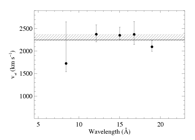
The horizontal line at 2250 km/s represents the literature value which we use for the profile fitting. When we actually fit a terminal velocity value to these five data, we find 2300 +/- 70 km/s (68% confidence) - represented here by the cross-hatched region.
last modified: 19 February 2009