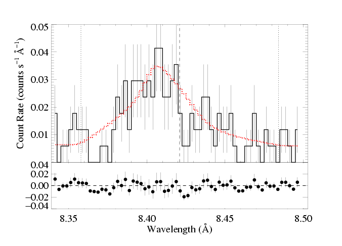
Mg XII 8.421 Angstroms

Models with isotropic porosity

Note: Both MEG and HEG are being fit simultaneously

Same continuum fit as we used for the non-porous models: n=2, best-fit norm=1.65e-3.

Note that the opacity bridging law used for these isoporosity fits is Rosseland.

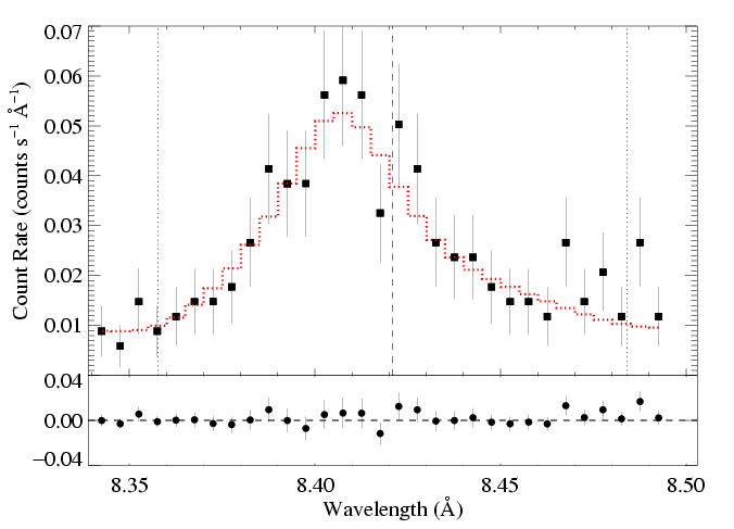
[8.34:8.50]
v_inf=2250
β=1
powerlaw continuum, n=2; norm=1.65e-3
q=0
h_inf=0.00 +/- (0.00:1.77) and for 90%
confidence, (0.00:4.32)
taustar=1.21 +/- (0.77:1.75)
u_o=0.756 +/- (0.660:0.885)
norm=2.95e-5 +/- (2.71e-5:3.19e-5)
rejection probability = 14% (C=186.53; N=188)

Note that while the confidence limit determination on the terminal porosity length, h_inf, is robust, the confidence limit determinations on taustar and u_o are not; with h_inf free while calculating models on a taustar and/or u_o grid, the fit often doesn't even converge to one as good as the corresponding non-porous case. We thus are quoting the confidence limits for the strictly non-porous case for these two model parameters. But, the upper limit on taustar must be higher, since very high values of the porosity length are allowed. (The plot below shows that it is basically unconstrained.)

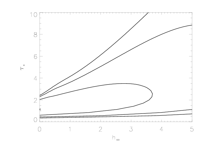
Here are the 68%, 90%, and 95% joint confidence limits on h_inf and taustar based on fitting the MEG and HEG data together. The asterisk represents the best-fit model, shown as the red histograms on the above two plots.

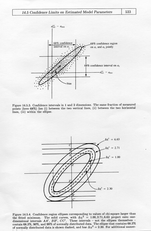
If large porosity lengths are allowed (which they are, according to the fit statistic criterion), then taustar is unconstrained. Note that the confidence limits on h_inf listed in the table above seem to be underestimated, based on the map of 2-D parameter space, although it could be a function of the joint probabilities (again, the situation shown graphically in Numerical Recipes).

Forcing a fit with taustar=4:

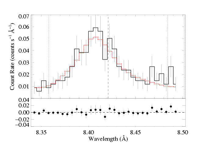
[8.34:8.50]
v_inf=2250
β=1
powerlaw continuum, n=2; norm=1.65e-3
q=0
h_inf=3.14 +/- (1.67:5.58) and for 90%
confidence, (1.09:8.05)
taustar=4
u_o=0.726 +/- (0.660:0.809)
norm=3.01e-5 +/- (2.7e-5:3.2e-5)
rejection probability = 16% (C=189.17; N=188)

As the confidence limit contour plot, above, showed, this higher optical depth model provides only a slightly worse fit than the global best-fit model with zero porosity length. In fact, it has ΔC~2.6, which implies that the non-porous model is preferred only at about the 90% level. We see from the fitting, though, that very large terminal porosity lengths are required in order to accommodate taustar=4 (which is our estimate of the optical depth value implied by the literature mass-loss rate). At the upper end, this parameter is basically unconstrained, but the lower bounds are pretty tight. At 90% confidence, the terminal porosity length is >1.

Next, we fit an anisotropic porosity model to the data.

Back to main page.

last modified: 8 May 2008