Determination of the fit parameter uncertainties
Using the baseline analysis (no porosity) case as an example
For the two fitted parameters (uo and taustar), we have:
taustar = 1.97 +/- (1.63:2.35)
uo = 0.655 +/- (0.605:0.725)
The values in the parentheses, after the "+/-" symbol, are the 68% confidence limits (lower and upper) of the parameter in question. (Note, they are not the uncertainties themselves, rather they are the best-fit value minus the negative uncertainty and the best-fit value plus the positive uncerainty. In other words, we can say with 68% confidence that the value of taustar for this line lies between 1.63 and 2.35.)
The best-fit values come from minimizing the maximum likelihood fit statistic, Cash's "C statistic." To determine the uncertainties - or, more accurately, the confidence limits - on the fit parameter values, we use the "error" command in XSPEC, which essentially calculates the run of fit statistic values as the parameter in question is varied. For each trial value of this parameter, all other important parameters are free to take on any value. Sometimes we use "steppar" which is more exact than "error" and also is the instrument of choice when we want to explore joint probability distributions between two or more parameters (see below).
The confidence limits are given by the crieterion that, for each model with parameter values i,j, ΔCij = Cij - Cmin has to be less than some particular value for a given confidence limit (e.g. ΔC = 2.3 corresponds to the 68% confidence limit for the joint probability distribution of two model parameters of interest; but when examining one parameter at a time, the 68% confidence limit is given by ΔC = 1.0). Note that there are always going to be different, more or less equally valid, ways of drawing confidence limit contours in model parameter space such that the space enclosed has a 68% chance of containing the true parameter values. In practice, how this is done will depend on how many parameters - and their joint probability distribution - are being examined at a given time. The relevant issues are discussed in Ch. 14 of Numerical Recipes, and this particular issue is described in Fig. 14.5.3.
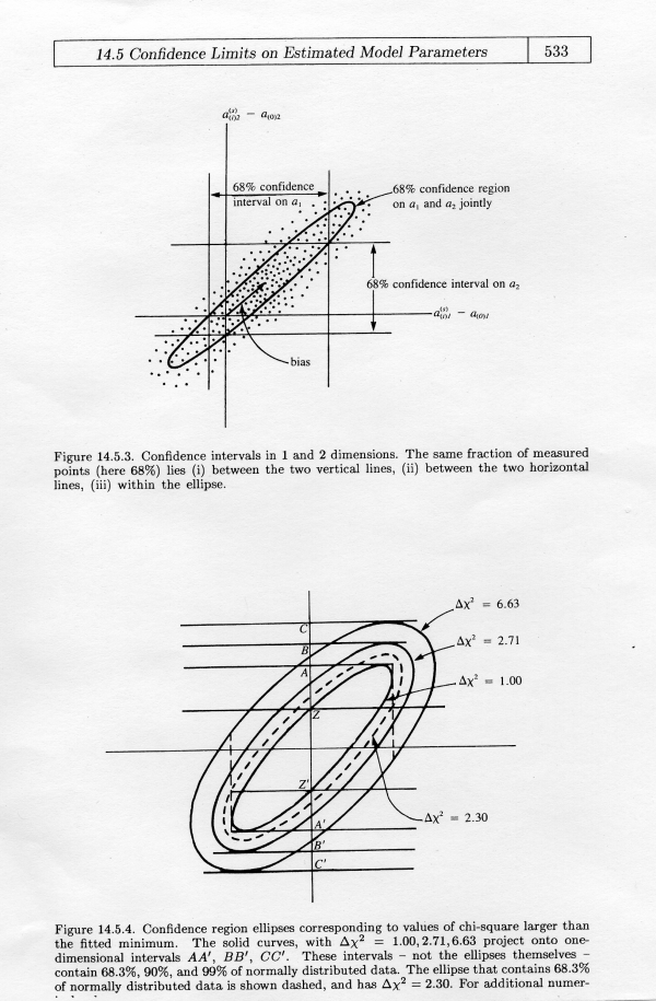
When two model parameters are correlated - as taustar and hinf are - it is advisable to place confidence limits on the two parameters jointly. One can then project the extremes of a given confidence contour onto each axis. The single parameter confidence range thus determined will generally be greater than the the range determined by assessing ΔC as a single parameter is varied (because some of the wider range is excluded for certain values of the second parameter; again, see the figure from Numerical Recipes). To account for the correlated nature of the two primary profile model parameters we are investigating - when fitting porous models, we generally will examine and plot the 2-D parameter space confidence contours, as shown below. However, when tabulating the 68% confidence limits on the entire set of fitted model parameters, we will generally examine each parameter, one at a time, using ΔC = 1.0 while varying each parameter in turn. Note though that at each point in these one-dimensional parameter studies, when we fit a model and minimize C, we allow the other physically meaningful parameters to be free.
We draw contours in the parameter space based on the ΔC values, and the projection of the relevant contour onto each parameter axis gives the corresponding confidence limit of that parameter, accounting for its joint distribution with the other plotted parameter. For example, here is the confidence limit contour plot for our baseline model fit:
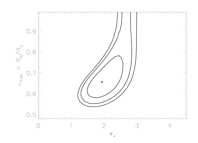
The two free parameters were taustar and uo (since the baseline model does not include porosity). The asterisk represents the best-fit model (shown at the top of the main page), and the contours enclose the 68%, 90% and 95% confidence limits, respectively (from interior to exterior). You'll note that the maximum extent of the projections of the 68% confidence contour onto each of the two axis corresponds to values somewhat larger than the quoted uncertainties at the top of this page (where one parameter at a time is assessed). This is shown graphically, below:
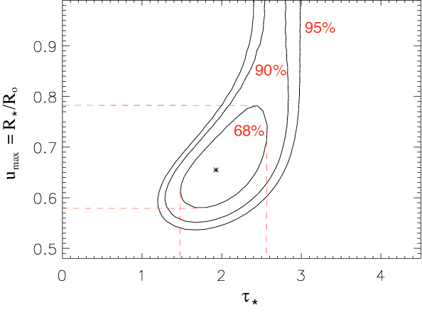
For example, note that 1.48 < taustar < 2.55 with 68% confidence here, when we take the joint probability distrubution of taustar along with uo into account. When we draw the 68% confidence limits simply looking at the variation of C with taustar by itself, we find the values quoted at the top of the page: 1.63 < taustar < 2.35. This is the issue illustrated in Fig. 14.5.3 of Numerical Recipes.
Note that while we can simply calculate the confidence limits on each parameter one at a time, looking at the joint probability distribution in this way allows one to examine the interplay between the effects of the two free parameters. In the plot above, one can see that there is a mild trade-off between optical depth and the minimum radius of x-ray emission. In general, we will quote 68% confidence limits based on an assessment of each parameter individually; however, we will graphically examine the joint probability distributions of the major parameters as well.
Finally, note that we use uo and umax interchangably, and that they're equal to the reciprocal of the minimum radius of X-ray emission, expressed in units of stellar radii.
Back to main page.
last modified: 22 April 2008