Global fits
Analysis of the entire 91 ks observation
2-temperature thermal model with non-solar abundances
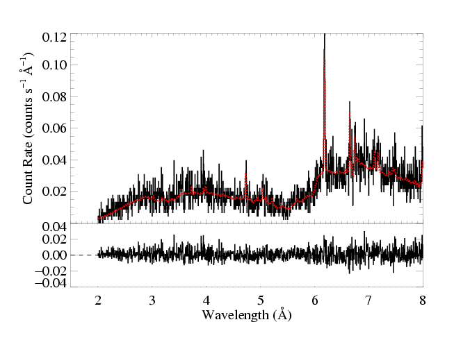
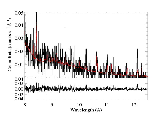
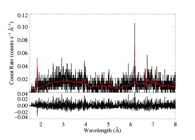
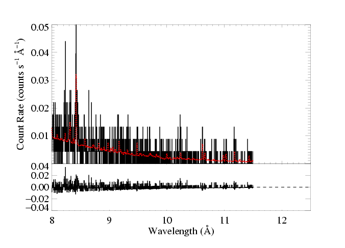
We use the bapec model - the state-of-the-art optically thin, coronal equilibrium thermal emission model. Its free parameters are temperature, emission measure, metallicity, and the Gaussian width of the lines. This last parameter isn't too important, as the lines are unresolved. We specify the model as: (bapec + bapec)*wabs which accounts for two different thermal component (each with their own temperature and emission measure, but with metallicity and line broadening parameters tied together), and to account for interstellar attenuation (the H column density is the sole free parameter of that model component). We fit the MEG (top two panels below) and HEG (bottom two) simultaneously, and plot the best-fit model on the data, with the fit residuals shown below. For clarity, we break both the MEG and HEG spectra into two sections. The axis ranges are the same for the pairs of plots. Note that "+/-" uncertainties are actually 68% confidence ranges for the specified parameters.
|
[2.0:12.5] MEG
[1.5:11.5] HEG kT1 = 1.00 +/- (0.97:1.04) keV abundance = 0.39 +/- (0.37:0.41) solar velocity = 0.0 +/- (0:49) km/s norm1 = 3.82e-3 +/- (3.43e-3:4.28e-3) kT2 = 4.16 +/- (4.05:4.27) keV abundance = 0.39 solar velocity = 0.0 km/s norm2 = 1.72e-2 +/- (1.68e-2:1.75e-2) NH = 1.19e22 +/- (1.15e22:1.22e22) χ2 = 11428 (N=12196) flux [0.3:10 keV] = 1.48e-11 erg/s/cm2 unabsorbed flux = 3.04e-11 erg/s/cm2 |
The fit is formally good, using chi squared with Churazov weighting. And it looks pretty good, both in the lines and the continuum. The biggest discrepancy appears to be the model's overprediction of the Fe XXV line and underprediction of the Si XIV Lyα line at 6.18 A. This may indicate the need to add a third model component (allowing for a small amount of hotter plasma with a corresponding downward adjustment of the current second component's temperature may increase the Si XIV line flux in the model, while maintaining the good fit to the continuum but lessening the Fe XXV flux). On the other hand, I haven't quantified the discrepancy between the model and data line fluxes, yet.
Keep in mind, though, that the formal errors on the model parameters are quite tight - unrealistically so, in my opinion. This tends to be the case when one has thousands of bins and a relatively simplified model.
We can also compare this fitting result to Marc's similar model-fitting using ISIS. Converting his results (8Aug08 email), which used chi square as the fit statistic and adaptively smoothed the data, to the same units we use here, we have:
kT1 = 1.20 +/- (1.14:1.33) keV
abundance = 0.35 (Fe) and 0.70 (Si) +/- (0.31:0.40; 0.65:0.76) solar
velocity = 131 +/- (0:201) km/s
norm1 = 1.49e-3 +/- (1.35e-3:1.72e-3)
kT2 = 5.54 +/- (5.40:5.99) keV
abundance = 0.35 (Fe) and 0.70 (Si) solar
velocity = 131 km/s
norm2 = 1.38e-2 +/- (1.33e-2:1.39e-2)
NH = 0.98e22 +/- (0.96e22:1.00e22)
Marc also gets a number density from the emission model, based on the altered (or not) f/i ratios. He finds an upper limit of 1.14e13. I haven't yet analyzed the R=f/i values derived from the fits to the individual complexes. But right now, we've got Si XIII in the low density limit quite securely, and S XV near it, with intermediate f/i values being marginally consistent with the lower limit of the line ratio derived from the data. But I don't think we can say that n_e < 1e14.
In any case, the ISIS results Marc reports are not formally consistent with the APEC/XSPEC results I report at the top of this page, but they are qualitatively consistent. The higher limit on the line broadening is one obvious difference. As is the higher Si abundance (note that the ISIS mvapec model allows for separate abundances for each specified element). Both temperatures are somewhat higher, but not hugely so. The normalizations are different, but that could entirely be a function of the different temperatures.
Questions I have based on these fit comparisons:
- How robust is the velocity broadening determination? Maybe the data aren't good enough to really differentiate anything below ~200 km/s.
- How robust is the Si abundance determination? Does it make sense to let individual abundances vary? Are both ISIS and XSPEC assuming the same standard solar abundances?
- What X-ray fluxes (on [0.3:10 keV]) are implied by the ISIS fits?
These global fits can be repeated for the subsets of the observation: pre-flare, flare, and post-flare intervals and we can look for statistically significant changes in the model parameters:
Pre-flare analysis
Flare analysis
Post-flare analysis
Back to the main page.
last modified: 12 April 2009