Global fits
Analysis of the pre-flare portion of the observation
The first 48 ks of the observation is analyzed here.
2-temperature thermal model with non-solar abundances
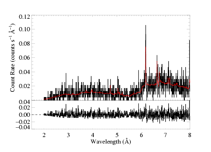
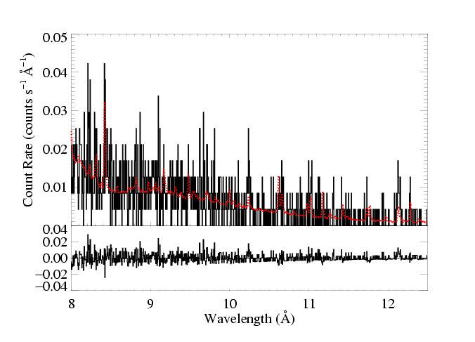
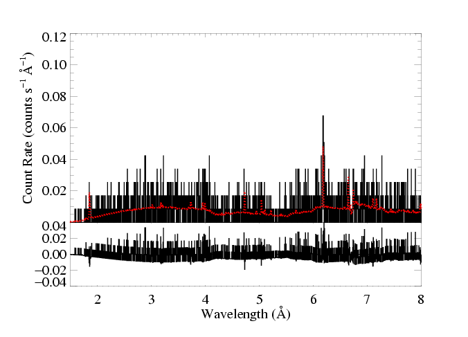
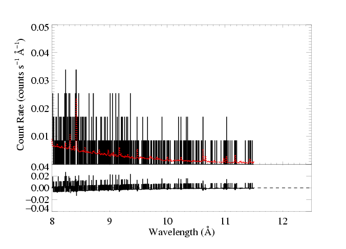
We use the same bapec (bapec + bapec)*wabs model we used to analyze the total observation's spectrum. We fit the MEG (top two panels below) and HEG (bottom two) simultaneously, and plot the best-fit model on the data, with the fit residuals shown below. For clarity, we break both the MEG and HEG spectra into two sections. The axis ranges are the same for the pairs of plots, and also the same we used for the total observation, to facilitate fair comparisons. Note that "+/-" uncertainties are actually 68% confidence ranges for the specified parameters.
|
[2.0:12.5] MEG
[1.5:11.5] HEG kT1 = 0.95 +/- (0.89:1.00) keV abundance = 0.26 +/- (0.24:0.28) solar velocity = 82 +/- (0:135) km/s norm1 = 4.13e-3 +/- (3.47e-3:4.90e-3) kT2 = 3.10 +/- (2.97:3.24) keV abundance = 0.26 solar velocity = 82 km/s norm2 = 1.22e-2 +/- (1.17e-2:1.28e-2) NH = 1.19e22 +/- (1.14e22:1.22e22) χ2 = 11136 (N=12196) flux [0.3:10 keV] = 7.97e-12 erg/s/cm2 unabsorbed flux = 1.95e-11 erg/s/cm2 |
The fit is formally good, using chi squared with Churazov weighting. And it looks pretty good, both in the lines and the continuum. The flux level is clearly lower than for the observation as a whole (the y-axis limits are the same here as for those plots). The spectrum is also softer, and the model fitting shown here demonstrates that this is entirely in the hotter component, which is only 3/4 as hot and 2/3 as strong as the hot component in the fit to the entire dataset. The overall flux is almost exactly a factor of 2 lower, the unabsorbed flux ratio isn't quite that big.
Compare these results to those from the flare and post-flare sections of the observation.
Back to the main page.
last modified: 12 April 2009