ζ Pup: XMM RGS line-profile analysis
The results presented here (February 2012) are still preliminary. Maurice has re-reduced the data using the latest software and calibration files. The results can be compared to those from the earlier (2010) reduction. We are concerned here with systematic wavelength errors and fit quality in addition to the science issues.
The data shown here were reduced by Maurice in January 2012, and include all GO and GTO observations. The effective exposure times are 846.2 ks for RGS1 and 841.8 ks for RGS2.
Comparisons can be made to these older, and extensive, fits to the Chandra data and also to a corresponding page of Chandra fit results analogous to the RGS fits shown on this page (i.e. also intended for paper II; same focus on porosity, and on high S/N unblended lines).
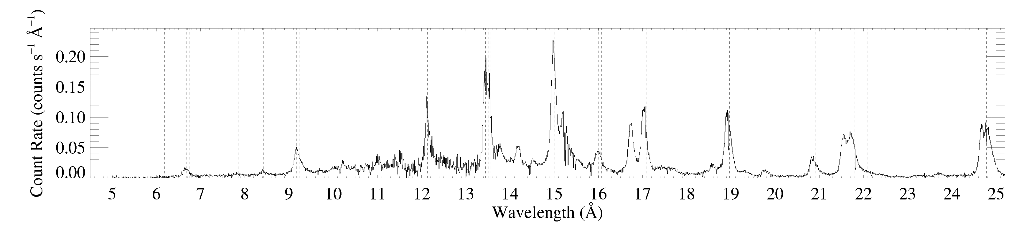
The entire RGS spectrum
RGS1

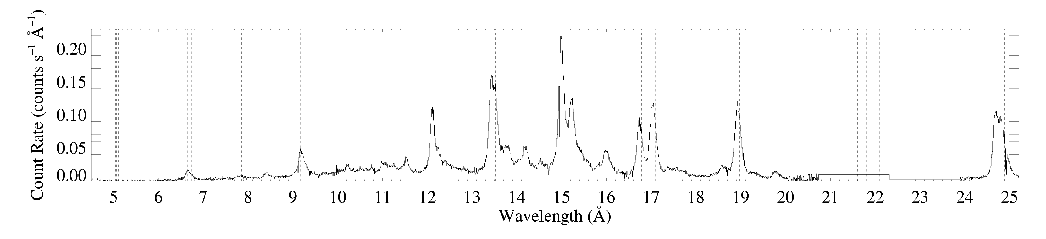
RGS2

On a somewhat narrower wavelength range, for direct comparison with the Chandra data [RGS1, RGS2]
From working with the previous reduction, we know that there are really only four unblended lines suitable for profile fitting: Ne X Lyα at 12.134 A, Fe XVII at 15.014 A, O VIII Lyα at 18.969 A, and N VII Lyβ at 20.910 A.
We fit the power-law continuum simultaneously (unlike with Chandra data) and also use chi-square with Churazov weighting (again, in contrast to our procedures with Chandra data).
Line-by-line results
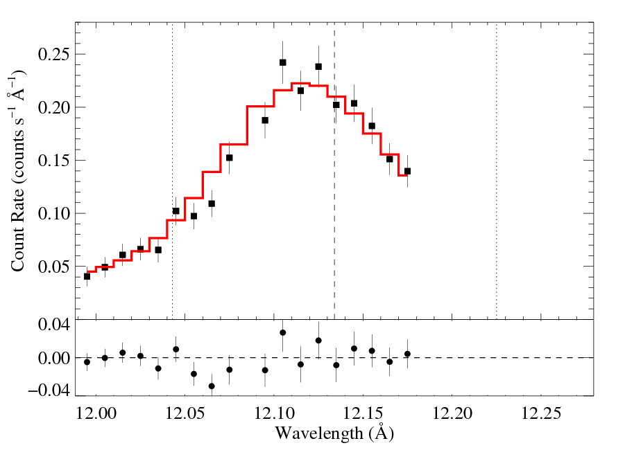
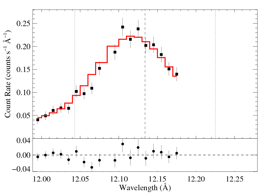
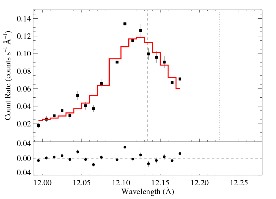
12.134 Angstroms: Ne X
Non-porous: RGS1+2
|
[11.98:12.18]
vinf = 2250 β = 1 powerlaw continuum, n = 2; norm = 1.57e-3 q = 0 hinf = 0 taustar = 1.67 +/- (1.47:1.92) Ro = 1.54 +/- (1.38:1.68) shift = 0 norm = 3.05e-4 +/- (2.98e-4:3.13e-4) chisq = 47.72 for N = 37 |
Note that the reduced chi square isn't that bad -- 1.45; for only a 95% rejection probability. (The formally good fit is due, in some sense, to the relatively low signal-to-noise in this line.) So, we can formally use the chi square statistic, and confidence limits on single parameters correspond to Delta chi square = 1, as is usual.
Compare these results to the analogous model fit to the same line in the Chandra spectrum. There is quite good agreement (taustar values disagree by about 20%, just about the formal confidence limit range).
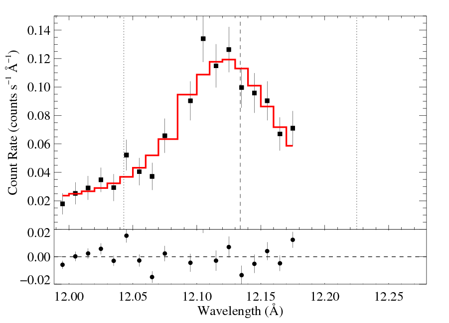
Next: Fitting the same data with the same model, we allowed the shift parameter to be free:
Non-porous: RGS1+2, shift free
|
[11.98:12.18]
vinf = 2250 β = 1 powerlaw continuum, n = 2; norm = 1.56e-3 q = 0 hinf = 0 taustar = 1.19 +/- (0.19:2.78) Ro = 1.62 +/- (1.01:1.74) shift = -2.45 +/- (-11.93:3.86) norm = 3.04e-4 +/- (2.96e-4:3.15e-4) chisq = 47.67 for N = 37 |
A best fit of -2.45 mA was found, but with a chi square improvement of less than one. In fact, the 68% confidence range on the shift is -11.9 to +3.85 mA -- quite large. And furthermore, when shift is allowed to be free, the other parameters (especially taustar) have significantly expanded confidence ranges (e.g. 0.19 to 2.78 at 68% confidence for taustar). Clearly, the range of plausible shifts is significantly narrower than the formal confidence range. Finally, with the "best-fit" shift of -2.45 mA, the best-fit taustar is reduced by about 30%, to 1.19.
Note: here and above, the RGS1 and RGS2 spectra are coadded for the plots (though not for the fitting). For the other lines, below, we will show them separately.
Now, we will fit the RGS1 and RGS2 separately for this same line (and with the same non-porous model), first, without any imposed wavelength shift.
Non-porous: RGS1
|
[11.98:12.18]
vinf = 2250 β = 1 powerlaw continuum, n = 2 norm = 2.39e-3 +/- (1.41e-3:3.38e-3) q = 0 hinf = 0 taustar = 0.66 +/- (0.29:1.38) Ro = 1.20 +/- (1.01:1.41) shift = 0 norm = 2.64e-4 +/- (2.38e-4:2.91e-4) chisq = 10.82 for N = 18 |
Hmmm, pretty low taustar, but big error range. These data look somewhat different than the mean profile. The RGS1 data are noisier looking than the RGS2 data (you can see it around 12 A in the big plots at the top).
Non-porous: RGS1, shift free
|
[11.98:12.18]
vinf = 2250 β = 1 powerlaw continuum, n = 2 norm = 2.49e-3 +/- (1.41e-3:3.38e-3) q = 0 hinf = 0 taustar = 0.33 +/- (0.00:1.54) Ro = 1.22 +/- (1.01:1.46) shift = -3.29 +/- (-11.4:6.34) norm = 2.60e-4 +/- (2.38e-4:2.91e-4) chisq = 10.75 for N = 18 |
So, the shift is not well-constrained, but the best-fit value is negative (though consistent with zero). And the effect is to lower taustar (since line asymmetries due to absorption can now be mimicked by a simple shift), and to broaden the confidence limits of other parameters.
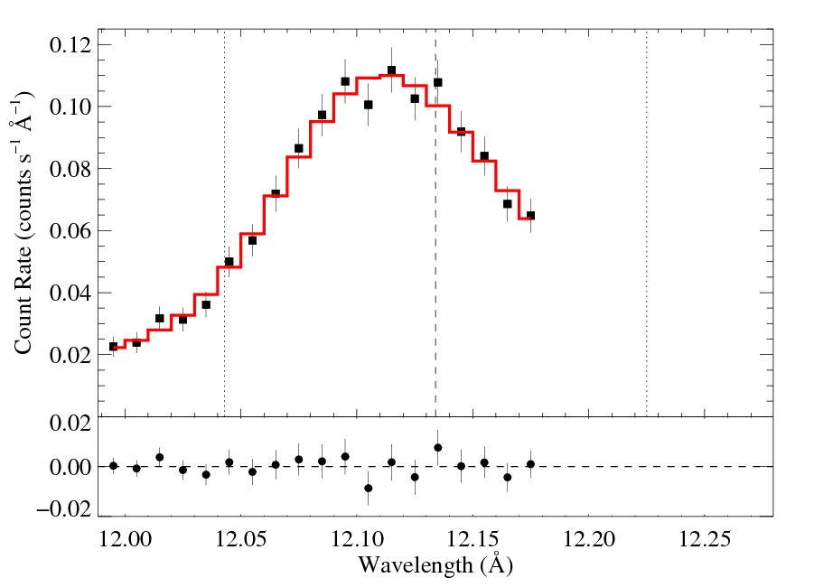
Non-porous: RGS2
|
[11.98:12.18]
vinf = 2250 β = 1 powerlaw continuum, n = 2 norm = 1.44e-3 +/- (1.14e-3:1.74e-3) q = 0 hinf = 0 taustar = 1.81 +/- (1.59:2.06) Ro = 1.61 +/- (1.43:1.76) shift = 0 norm = 3.10e-4 +/- (3.02e-4:3.18e-4) chisq = 24.04 for N = 19 |
The taustar value is significantly higher than for the RGS1 fit. The data quality looks better, too.
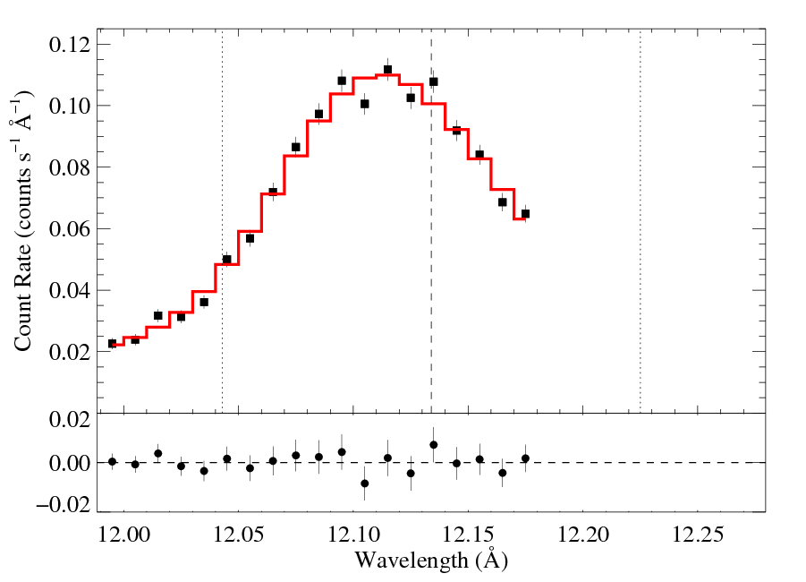
Non-porous: RGS2, shift free
|
[11.98:12.18]
vinf = 2250 β = 1 powerlaw continuum, n = 2 norm = 1.41e-3 +/- (1.07e-3:1.72e-3) q = 0 hinf = 0 taustar = 1.05 +/- (0.15:2.94) Ro = 1.69 +/- (1.01:1.80) shift = -3.95 +/- (-13.2:3.83) norm = 3.08e-4 +/- (2.99e-4:3.19e-4) chisq = 23.87 for N = 19 |
Again, a modest, negative shift is preferred, and again it leads to a lower taustar value and larger confidence regions.
Note that even though the best-fit shift values are very similar for the two datasets, the physical model parameters of these fits are rather different. Hence, the above dual RGS1+2 fit with the shift free provides a much worse fit than the fits to the individual datasets. And it makes it hard to know how best to combine the two datasets (both shifts could be free and independent in a combined fit).
On the other hand, the RGS2 data is better -- higher S/N, significantly. So, maybe only the RGS2 data should be used (even if we can "correctly" apply independent shifts in a combined fit, the fit will be dominated by the higher S/N dataset.
Non-porous: RGS1+2, relative shift of RGS2 = RGS1 + 5 mA
Going back to the combined spectra, here we test models for which a systematic +5mA offset is imposed on the RGS2 spectrum (in accord with some calibration studies -- on the XMM calibration document site and specifically, p. 17 of this 2011 document). We are not sure if these systematic offsets have been included in the latest version of SAS, so we are experimenting with imposing them via independent fitting of the shift parameter for the two datasets. We are assuming a +/-2mA systematic offset overall, so we test the following combinations of RGS1,RGS2 offsets: -2,+3mA; 0,+5mA; +2,+7mA; +4,+9mA.
We do not show the fits for now, just list the results:
-2,+3: taustar=2.58 (2.16:2.79), chi-sq=59.75
0,+5: taustar=2.97 (2.64:3.23), chi-sq=61.59
+2,+7: taustar=3.44 (3.13:3.76), chi-sq=65.89
+4,+9: taustar=4.05 (3.69:4.45), chi-sq=72.34
Compare these to the fit with no shift (shown above):
0,0: taustar=1.67 (1.47:1.92), chi-sq=47.72
This unshifted fit is significantly better. (And the fit with a free (but tied RGS1+2) fit, also shown above, is on par with the unshifted fit. So, the tentative conclusion here is that a relative shift of +5mA for the RGS2 w.r.t. RGS1 is not correct.
And the tentative recommendation for this line overall, is to use just the RGS2 data (and go with the fit that allows a free shift parameter).
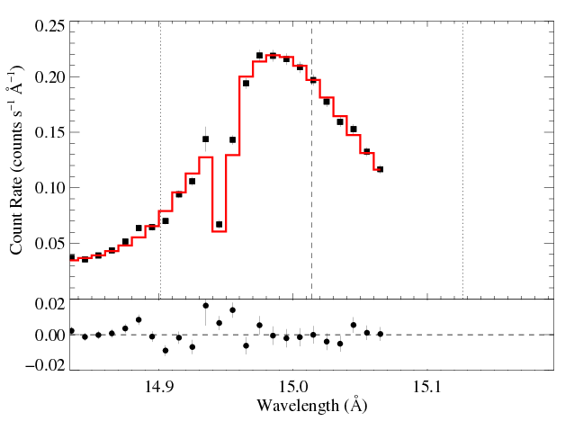
15.014 Angstroms: Fe XVII
Non-porous: RGS1+2
RGS1
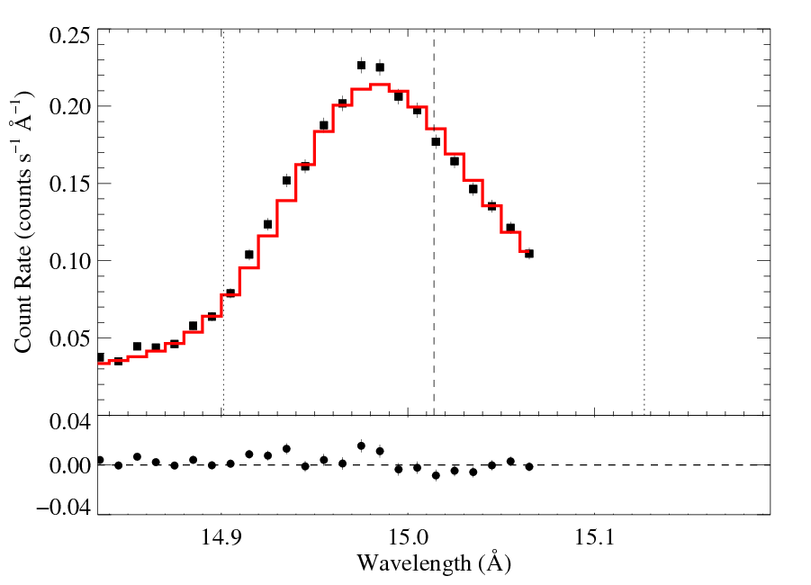
RGS2 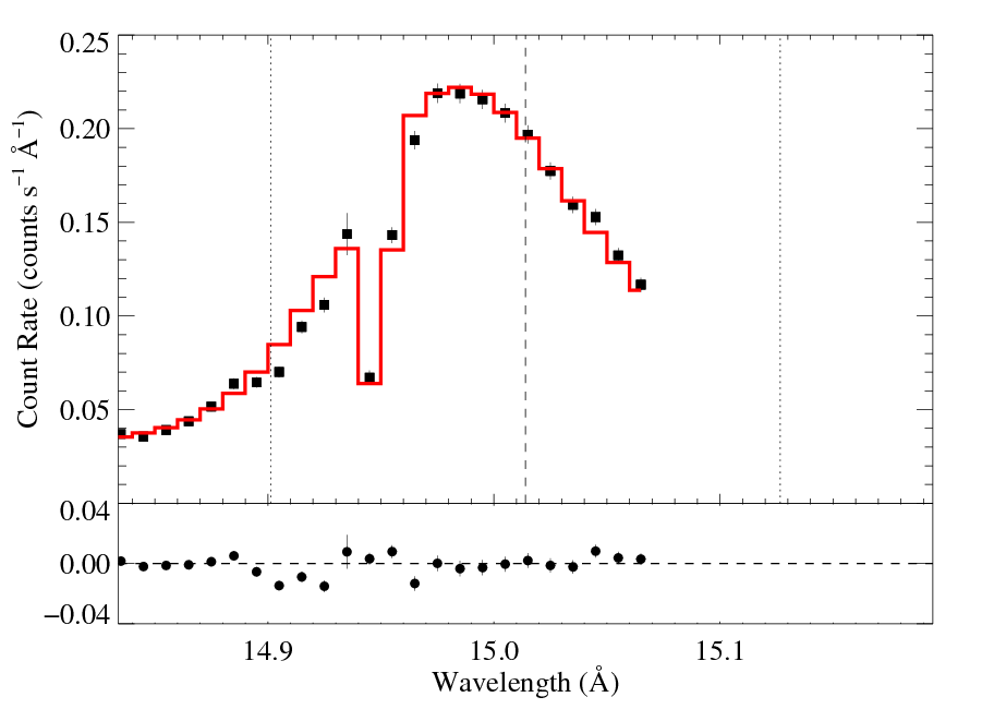
|
[14.80:15.07]
vinf = 2250 β = 1 powerlaw continuum, n = 2 norm = 3.13e-3 +/- (:) q = 0 hinf = 0 taustar = 1.77 +/- (:) Ro = 1.57 +/- (:) shift = 0 norm = 6.39e-4 +/- (:) chisq = 129.54 for N = 52 |
We show the two spectra separately, but they were fit simultaneously. That's the same model in both plots.
Note: Because the reduced chi square of this fit is >2, XSPEC won't compute the confidence limits on the model parameters. The chi square of the best fit model is high most likely because the formal error bars are so low, while the actual errors are probably dominated by systematics (which, of course, aren't included in the error bars). We will not worry about the formal confidence limits for now, as we are presently mostly interested in looking at fit quality and how it changes when wavelength scale errors are accounted for and if data from the two detectors are fit separately.
Note: The low bin on the blue wing is due to the low sensitivity of a particular detector pixel, and is thought to be well calibrated. We repeated this fit with the bin eliminated and got a very similar fit, with a very similar fit quality.
Compare the results of this fit to those derived from the same line in the Chandra spectrum. The results are quite consistent.
Next: we will investigate whether better fits can be achieved for one or the other datasets, fit individually, as we did, above, for Ne X.
Non-porous: RGS1, no shift
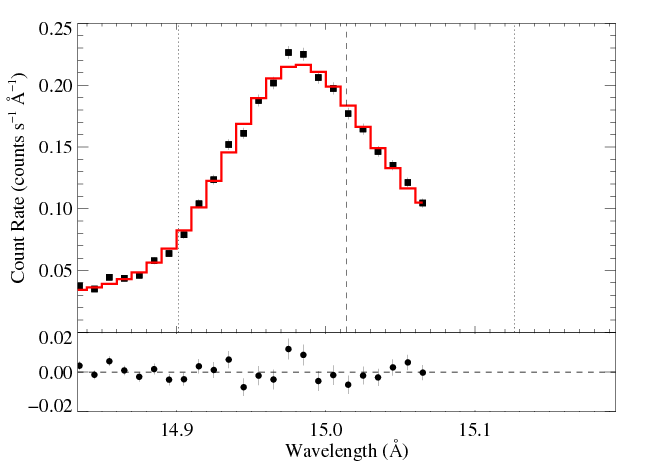
|
[14.80:15.07]
vinf = 2250 β = 1 powerlaw continuum, n = 2 norm = 3.19e-3 +/- (3.02e-3:3.32e-3) q = 0 hinf = 0 taustar = 2.30 +/- (2.14:2.50) Ro = 1.42 +/- (1.26:1.53) shift = 0 norm = 6.48e-4 +/- (6.41e-4:6.56e-4) chisq = 33.09 for N = 26 |
Non-porous: RGS1, shift free
|
[14.80:15.07]
vinf = 2250 β = 1 powerlaw continuum, n = 2 norm = 3.18e-3 +/- (2.96e-3:3.40e-3) q = 0 hinf = 0 taustar = 2.38 +/- (1.87:2.74) Ro = 1.39 +/- (1.18:1.55) shift = 0.32 +/- (-1.82:1.78) norm = 6.49e-4 +/- (6.41e-4:6.58e-4) chisq = 33.05 for N = 26 |
The shift is quite consistent with zero. The fit quality is good. The derived model parameters are a bit different than those from the combined RGS1+2 fit, shown above (but see the fits, below, with the independent shifts for the two detectors).
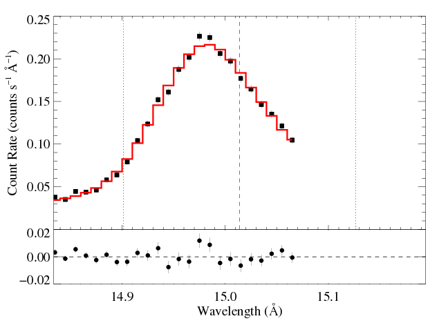
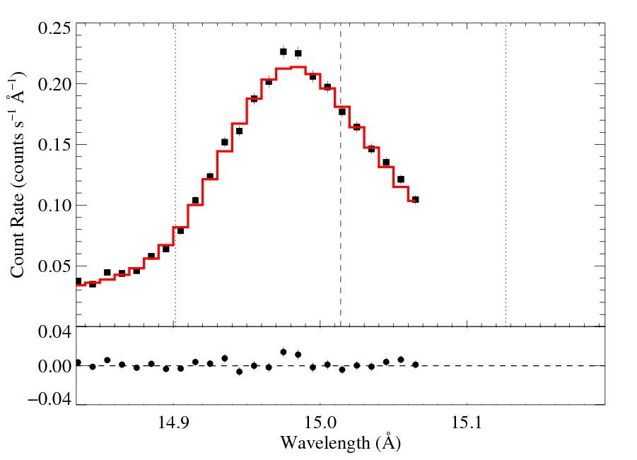
Non-porous: RGS2, no shift

|
[14.80:15.07]
vinf = 2250 β = 1 powerlaw continuum, n = 2 norm = 3.20e-3 +/- (:) q = 0 hinf = 0 taustar = 1.28 +/- (:) Ro = 1.61 +/- (:) shift = 0 norm = 6.25e-4 +/- (:) chisq = 47.88 for N = 26 |
Non-porous: RGS2, shift free
|
[14.80:15.07]
vinf = 2250 β = 1 powerlaw continuum, n = 2 norm = 3.21e-3 +/- (:) q = 0 hinf = 0 taustar = 1.79 +/- (:) Ro = 1.55 +/- (:) shift = 3.13 +/- (:) norm = 6.28e-4 +/- (:) chisq = 47.31 for N = 26 |
While the improvement to the fit with shift allowed to be a free parameter is not statistically significant, a larger value of shift is preferred over the unshifted model, and the other, physical parameter models are more in-line with those from the RGS1 fit when the this non-zero shift is used.
And next: we allow both dataset's shift parameters to be free simultaneously.
Non-porous: RGS1+2, both shifts free
RGS1
RGS2 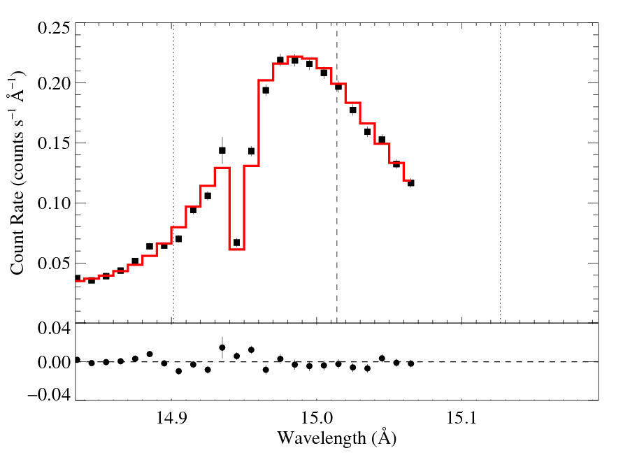
|
[14.80:15.07]
vinf = 2250 β = 1 powerlaw continuum, n = 2 norm = 3.18e-3 +/- (3.03e-3:3.33e-3) q = 0 hinf = 0 taustar = 2.22 +/- (1.75:2.55) Ro = 1.46 +/- (1.32:1.58) shift = -0.41,5.13 +/- (-2.62:0.97, 2.89:6.47) norm = 6.40e-4 +/- (6.34e-4:6.47e-4) chisq = 86.97 for N = 52 |
This fit is significantly better than the unshifted simultaneous fit to the same data, but still not formally good (though because Δχ2 < 2, XSPEC will calculate formal confidence limits).
The tentative recommendation is to use both the RGS1 and RGS2 data, and use the fit with both shifts free. Alternatively, we could use just the RGS1 data, with the shift free (which in any case is close to zero), which gives a formally good fit. Both of these approaches give similar results.
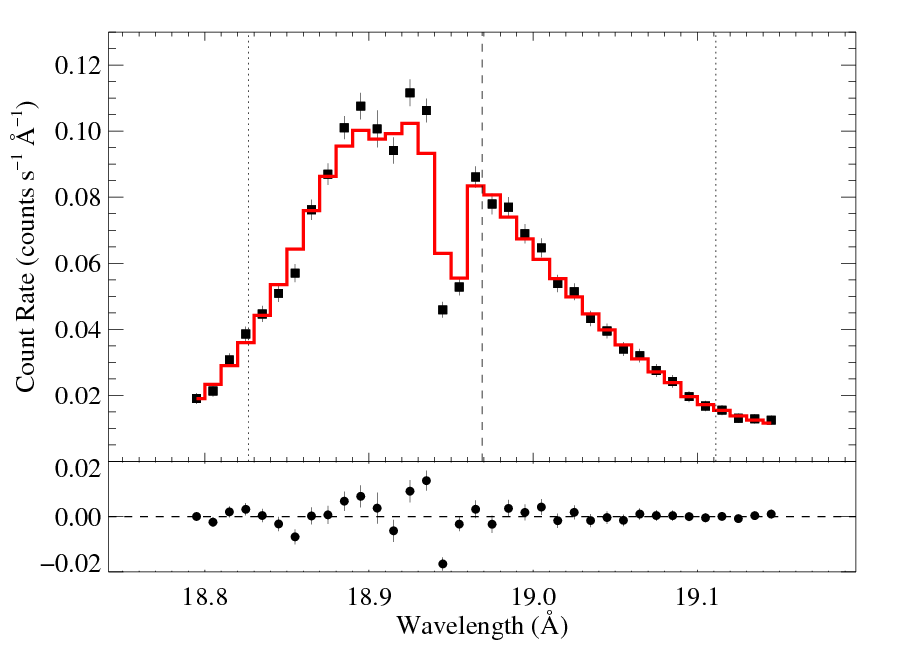
18.969 Angstroms: O VIII
Non-porous: RGS1+2
RGS1
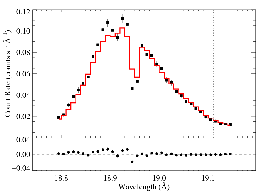
RGS2 
|
[18.78:19.15]
vinf = 2250 β = 1 powerlaw continuum, n = 2 norm = 9.77e-4 q = 0 hinf = 0 taustar = 3.14 Ro = 1.01 shift = 0 norm = 4.66e-4 chisq = 204.34 for N = 72 |
This fit -- with no shift allowed -- is quite poor. You can compare this result to the same sort of model fit to the Chandra spectrum. The results are similar, but we have to investigate the wavelength shift issue before drawing conclusions.
Rather than look at a single shift value for the combined RGS1+2 fit, let's first look at fits to the individual spectra.
Non-porous: RGS1, no shift

|
[18.78:19.15]
vinf = 2250 β = 1 powerlaw continuum, n = 2 norm = 5.43e-4 q = 0 hinf = 0 taustar = 3.68 Ro = 1.39 shift = 0 norm = 4.87e-4 chisq = 111.70 for N = 36 |
The fit is quite poor -- on par with the combined fit to both datasets. Let's see how much improvement we get with shift allowed to be a free parameter.
Non-porous: RGS1, shift free
|
[18.78:19.15]
vinf = 2250 β = 1 powerlaw continuum, n = 2 norm = 1.06e-3 q = 0 hinf = 0 taustar = 2.24 Ro = 1.72 shift = -6.61 norm = 4.70e-4 chisq = 96.16 for N = 36 |
A statistically significant improvement, but still not formally a good fit (which somewhat invalidates the assessment of how significant the improvement is). The best fit parameters are pretty different (even the continuum normalization level) than the shift = 0 fit, though taustar is still pretty high.
Non-porous: RGS2, no shift
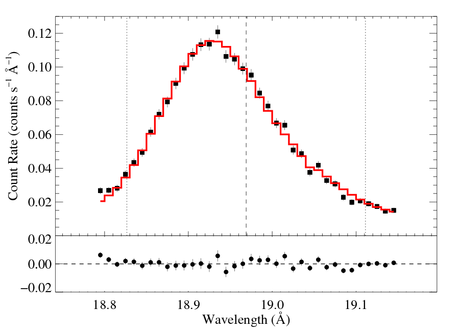
|
[18.78:19.15]
vinf = 2250 β = 1 powerlaw continuum, n = 2 norm = 1.42e-3 q = 0 hinf = 0 taustar = 2.63 Ro = 1.01 shift = 0 norm = 4.46e-4 chisq = 47.31 for N = 36 |
The fit is much better than either fit to the RGS1 data.
Non-porous: RGS2, shift free
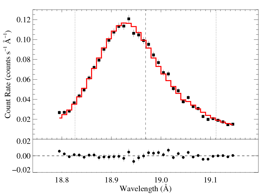
|
[18.78:19.15]
vinf = 2250 β = 1 powerlaw continuum, n = 2 norm = 1.60e-3 q = 0 hinf = 0 taustar = 2.44 Ro = 1.01 shift = -2.03 norm = 4.40e-4 chisq = 43.97 for N = 36 |
Not a hugely statistically significant improvement, but a formally good fit (as is, basically, the unshifted model, shown above this one).
But: while assessing the parameter confidence limits, I found a (much) better fit -- with a chi-square of 30.67. However: the shift found for this fit is unrealistically large (shift = -12.86). And it gives a very low taustar = 0.7 (no surprise -- the empirical blue shift of the line is accounted for in this model mostly by the wavelength shift/uncertainty, rather than a physical absorption effect). I wondered if the solution space was smooth or if maybe there were two regimes of good fits: high-shift, low-taustar vs. low-shift, high-taustar with a dis-allowed region in between. But running steppar on shift (with taustar and Ro free) showed a smoothly varying fit parameter trend with a global minimum between -13 and -12 mA for shift.
So, in principle, while we could impose an allowed range of shift values, there's no obvious way to objectively define such an allowed range based just on the behavior of this data alone. We could limit it to, say, shift > -5 mA, based on calibration documents. If we do that, here's the best-fit model:
Non-porous: RGS2, shift = -5 mA

|
[18.78:19.15]
vinf = 2250 β = 1 powerlaw continuum, n = 2 norm = 1.69e-3 +/- (1.52e-3:1.87e-3) q = 0 hinf = 0 taustar = 1.51 +/- (1.40:1.63) Ro = 1.59 +/- (1.53:1.65) shift = -5 norm = 4.37e-4 +/- (4.30e-4:4.44e-4) chisq = 37.35 for N = 36 |
OK, this fit is (also) good; better than the unshifted fit, worse than the fit with the shift completely free. And taustar has, unsurprisingly, an intermediate value. Unfortunately, taustar is quite sensitive to the value of shift, and specifically, varies by about a factor of two even just between shift = 0 and shift = -5 mA.
So, what should we do to assess taustar for this line? Should we use only the RGS2 data, which gives a much better fit than the RGS1 data? What kind of shift should we impose or allow?
At this point, I am not going to present fits to the combined RGS1 and RGS2 data with relative and absolute shifts free. The above two questions have to be resolved first.
The tentative recommendation is to use only the RGS2 data, which gives a better fit (and appears to have smaller systematics, though the statistical S/N seems similar for each dataset). And to only allow a shift as big as -5 mA. But there's some sensitivity (of taustar especially) to where we place this cut-off.
20.910 Angstroms: N VII
Note: there is almost no RGS2 data for this line, so we will look only at RGS1 data.
Non-porous: RGS1, no shift
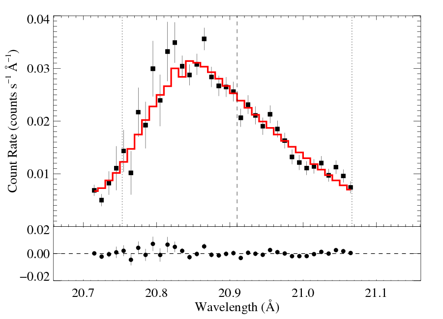
|
[20.70:21.07]
vinf = 2250 β = 1 powerlaw continuum, n = 2 norm = 9.05e-4 +/- (7.33e-4:1.13e-3) q = 0 hinf = 0 taustar = 4.93 +/- (3.90:5.59) Ro = 1.41 +/- (1.01:2.03) shift = 0 norm = 1.66e-4 +/- (1.56e-4:1.73e-3) chisq = 40.52 for N = 36 |
The fit is quite good (though mostly, I assume, because these data are relatively low S/N). The taustar value is high, as would be expected.
Non-porous: RGS1, shift free

|
[20.70:21.07]
vinf = 2250 β = 1 powerlaw continuum, n = 2 norm = 9.13e-4 +/- (7.41e-4:1.15e-3) q = 0 hinf = 0 taustar = 4.88 +/- (3.77:6.13) Ro = 1.37 +/- (1.01:2.04) shift = 0.22 +/- (-3.08:3.62) norm = 1.65e-4 +/- (1.56e-4:1.73e-4) chisq = 40.51 for N = 36 |
This fit is very similar, since the best-fit shift value is so close to zero. Note that even with shift allowed to be a free parameter, the confidence limits on the other parameters do not expand very much.
The tentative recommendation is to use this shift free fit to the RGS1 data.
last modified: 19 March 2012