ζ Pup: XMM RGS line-profile analysis
The results presented here (August 2011) are preliminary. Initially, we're exploring issues related to the model fitting and looking at some rudimentary results for taustar trends among the strong lines and the taustar vs. porosity-length tradeoff.
The data shown here were reduced by Maurice in 2010, and include all GO and GTO observations. A set of brief emails from him describing the reduction are available [14 June 2010 and 21 June 2010]. The effective exposure times are 767 ks for RGS1 and 763 ks for RGS2.
Comparisons can be made to these older, and extensive, fits to the Chandra data. New: and now there's a corresponding page of Chandra fit results analogous to the RGS fits shown on this page.
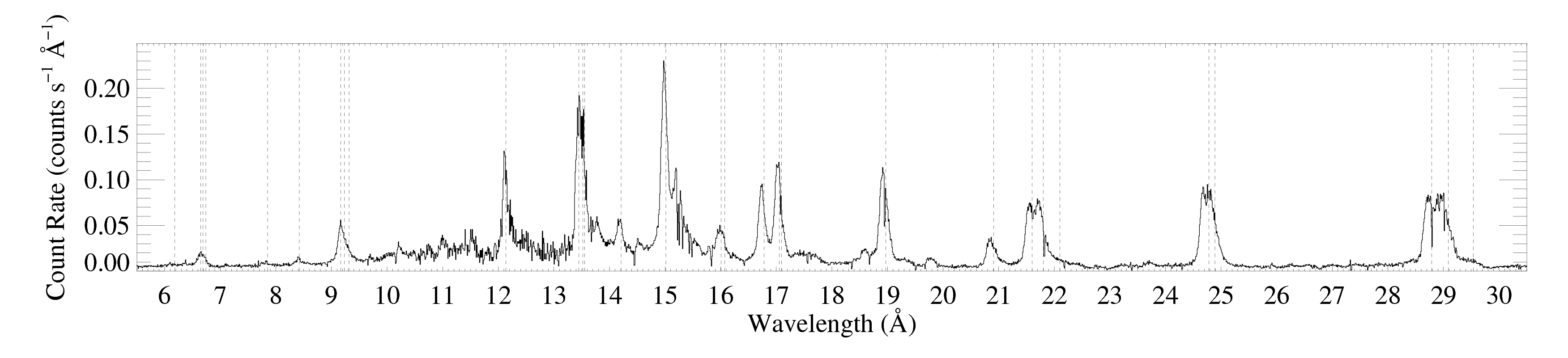
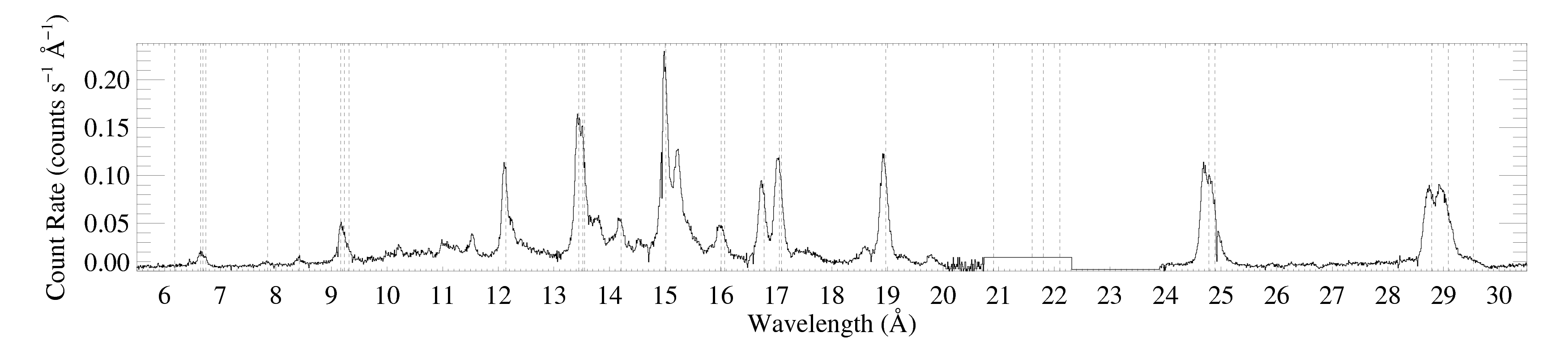
The entire RGS spectrum
RGS1
RGS2
Line-by-line results
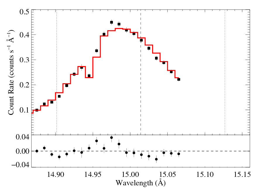
15.014 Angstroms: Fe XVII
We did some preliminary tests first, exploring the background, continuum fitting, optimal statistic and error weighting, and wavelength range over which to fit.
Below are the systematic fits of different model cases.
Non-porous

|
[14.80:15.07]
vinf = 2250 β = 1 powerlaw continuum, n = 2; norm = 3.23e-3 q = 0 hinf = 0 taustar = 1.84 +/- (1.69:1.99) Ro = 1.57 +/- (1.47:1.66) norm = 6.41e-4 +/- (6.28e-4:6.51e-4) chisq = 110.34 for N = 52 |
Note that the uncertainties on taustar and hinf assume delta chi square = 1, with the errors scaled up by 2.3 (so, in effect, we're using delta chi square = 2.3).
Compare these results to the analogous model fit to the same line in the Chandra spectrum.
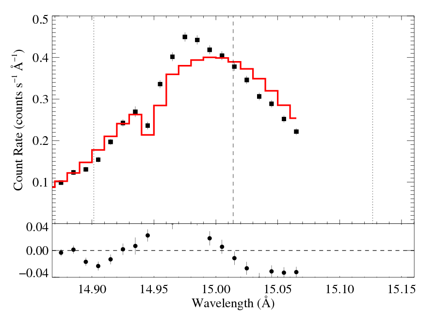
Anisotropic porosity
We test several values of hinf, using anisotropic porosity, employing the Rosseland bridging law (and with the numerical switch on). When the porosity length is treated as a free parameter, hinf=0 was preferred, with the non-porous fit parameters recovered (i.e. the data do not favor anisotropic porosity).
hinf = 0.5
|
[14.80:15.07]
vinf = 2250 β = 1 powerlaw continuum, n = 2; norm = 2.99e-3 q = 0 hinf = 0.5 (frozen) taustar = 3.41 Ro = 1.44 norm = 6.49e-4 chisq = 157.87 for N = 52 |
hinf = 1
|
[14.80:15.07]
vinf = 2250 β = 1 powerlaw continuum, n = 2; norm = 2.88e-3 q = 0 hinf = 1.0 (frozen) taustar = 4.89 Ro = 1.49 norm = 6.54e-4 chisq = 222.34 for N = 52 |
hinf = 5
|
[14.80:15.07]
vinf = 2250 β = 1 powerlaw continuum, n = 2; norm = 2.43e-3 q = 0 hinf = 5.0 (frozen) taustar = 33.40 Ro = 1.53 norm = 6.69e-4 chisq = 521.61 for N = 52 |
All three of these anisotropic porosity models (hinf = 0.5, 1, 5) produce poor fits from a formal statistical point of view (though the situation is ambiguous, quantitatively, because the best-fit model does not produce a formally good chi square) and qualitatively, visually, the venetian blind bump is apparent in the model at a level greater than what is seen in the data.
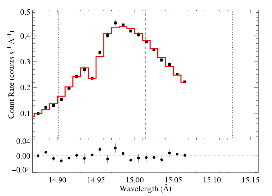
Isotropic porosity
Here we fit models with isotropic porosity (and still using the Rosseland bridging law), for the same set of fixed terminal porosity length values. Again, when hinf is allowed to be free, a best-fit value of zero is found, indicating the non-porous models are favored, though as can be seen below, for small porosity lengths, the quality of the model fits is roughly the same as for the non-porous model.
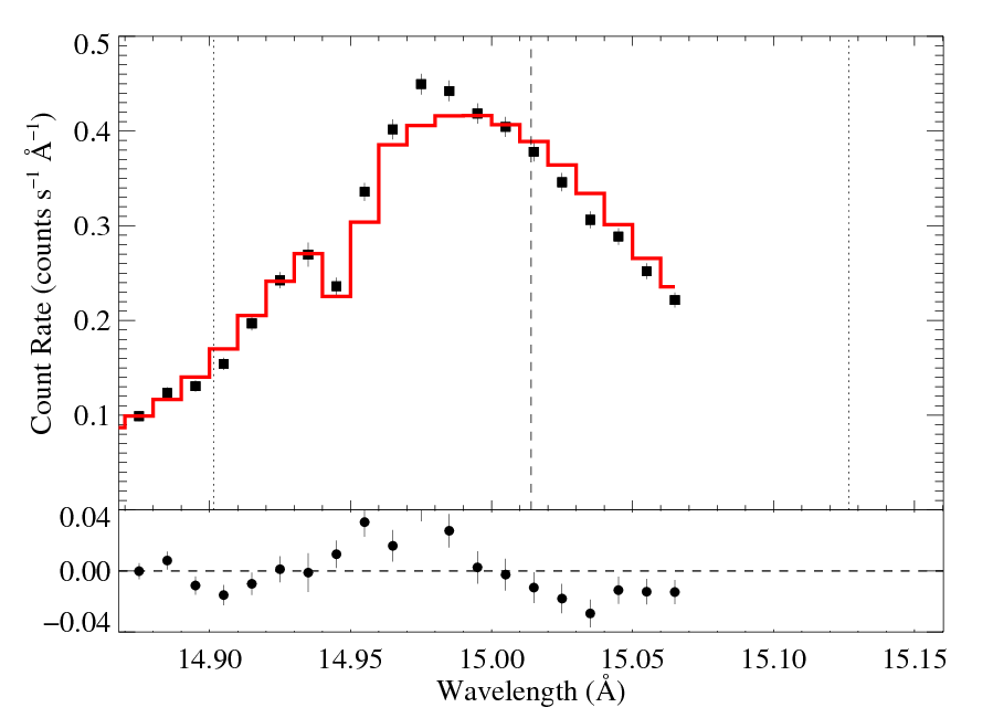
hinf = 0.5

|
[14.80:15.07]
vinf = 2250 β = 1 powerlaw continuum, n = 2; norm = 3.21e-3 q = 0 hinf = 0.5 (frozen) taustar = 2.11 +/- (1.93:2.31) Ro = 1.58 +/- (1.50:1.67) norm = 6.41e-4 +/- (6.32e-4:6.51e-4) chisq = 111.89 for N = 52 |
hinf = 1
|
[14.80:15.07]
vinf = 2250 β = 1 powerlaw continuum, n = 2; norm = 3.19e-3 q = 0 hinf = 1.0 (frozen) taustar = 2.44 +/- (2.21:2.71) Ro = 1.59 +/- (1.52:1.66) norm = 6.42e-4 +/- (6.32e-4:6.51e-4) chisq = 113.75 for N = 52 |
hinf = 5

|
[14.80:15.07]
vinf = 2250 β = 1 powerlaw continuum, n = 2; norm = 2.94e-3 q = 0 hinf = 5.0 (frozen) taustar = 10.63 +/- (8.85:13.20) Ro = 1.62 +/- (1.56:1.67) norm = 6.46e-4 +/- (6.37e-4:6.55e-4) chisq = 152.05 for N = 52 |
Here, for the isotropic porosity models, the first two models (with hinf = 0.5 and 1.0) are only very slightly worse than the non-porous model fit. Statistically, they are indistinguishable. Note that the actual taustar values found for these models tell us something -- they are only slightly higher than the non-porous best-fit model, implying that isotropic porosity has very little effect on the line profiles for porosity lengths less than unity. But, the high porosity model, with (hinf = 5) does produce a substantially worse fit (and a rather high value of taustar).
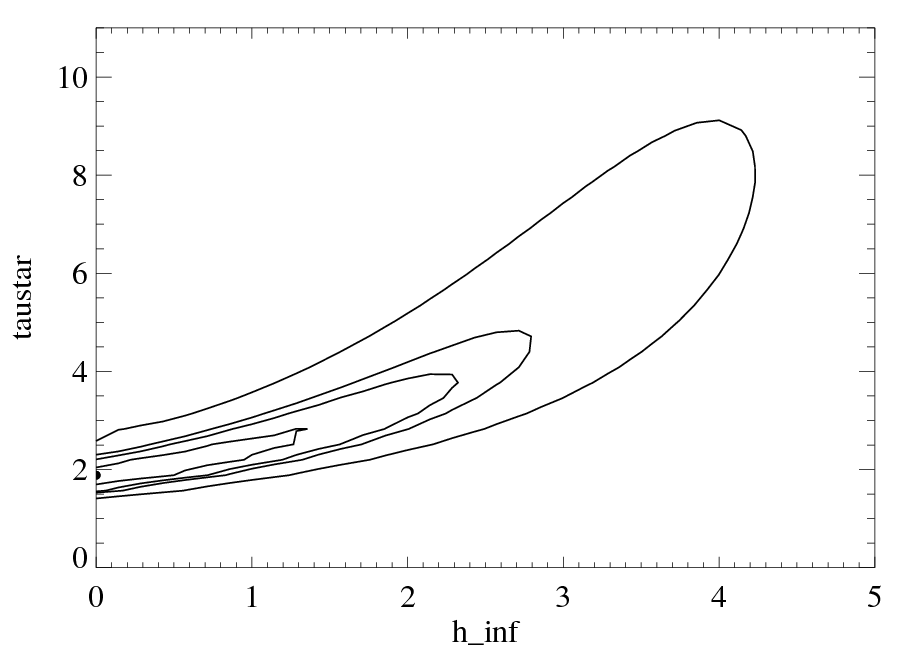
Confidence limits in taustar-hinf parameter space
|
Given the isotropic porosity model, and allowing hinf now to be a free parameter, along with the others, we can examine a 2-D grid of chi square values. The global best-fit model is denoted by the filled circle and the contours represent the formal 68%, 90%, and 95% confidence limits (with a scaling of 2.3 to correct for the formally poor fit of the best-fit model, as we have done above when evaluating confidence limits on individual parameters). The fourth, outermost contour is arbitrarily set at twice the value of the 95% contour, and its purpose is simply to trace out the quantitative tradeoff between the two parameters in the fit. (Note that Ro, along with the normalizations, is still a free parameter here even though it is not shown in this parameter space).
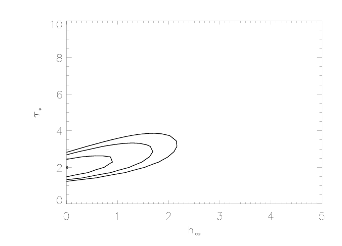
Here too, there is good agreement with the corresponding Chandra result.
18.969 Angstroms: O VIII
Note that we're treating the closely spaced Ly-alpha doublet as a single line, centered at the emissivity-weighted mean of the wavelengths of the two components.
Below are the systematic fits of different model cases. Same as above for the Fe XVII line at 15.014 A.
Non-porous
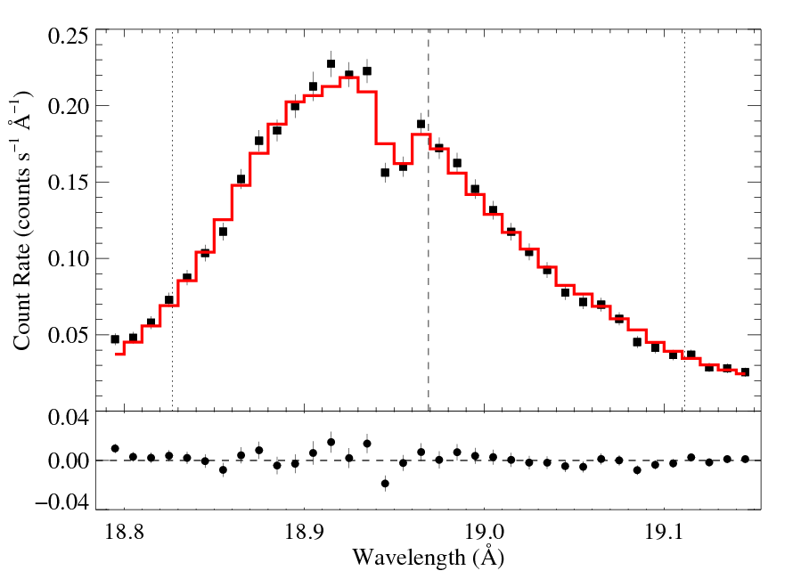
|
[18.78:19.15]
vinf = 2250 β = 1 powerlaw continuum, n = 2; norm = 9.35e-4 q = 0 hinf = 0 taustar = 3.10 +/- (2.80:3.29) Ro = 1.21 +/- (1.01:1.51) norm = 4.69e-4 +/- (4.61e-4:4.78e-4) chisq = 181.30 for N = 72 |
Note that the uncertainties on taustar and hinf assume delta chi square = 1, with the errors scaled up by 2.7 (so, in effect, we're using delta chi square = 2.7).
Compare these results to the analogous model fit to the same line in the Chandra spectrum. There is very good agreement.
Anisotropic porosity
When the porosity length is treated as a free parameter, hinf=0 was preferred, with the non-porous fit parameters recovered (i.e. the data do not favor porosity). Below, we test several values of hinf, using anisotropic porosity, as we did, above, for the Fe XVII line at 15.014 A.
hinf = 0.5
|
[18.78:19.15]
vinf = 2250 β = 1 powerlaw continuum, n = 2; norm = 5.82e-4 q = 0 hinf = 0.5 (frozen) taustar = 5.30 Ro = 1.36 norm = 4.80e-4 chisq = 256.90 for N = 72 |
hinf = 1
|
[18.78:19.15]
vinf = 2250 β = 1 powerlaw continuum, n = 2; norm = 4.09e-4 q = 0 hinf = 1.0 (frozen) taustar = 8.14 Ro = 1.43 norm = 4.84e-4 chisq = 335.33 for N = 72 |
hinf = 5
|
[18.78:19.15]
vinf = 2250 β = 1 powerlaw continuum, n = 2; norm = 2.52e-9 (note: unrealistic) q = 0 hinf = 5.0 (frozen) taustar = 73.43 Ro = 1.38 norm = 4.94e-4 chisq = 615.04 for N = 72 |
So, the anisotropic porosity models provide poor fits; even with modest terminal porosity lengths.
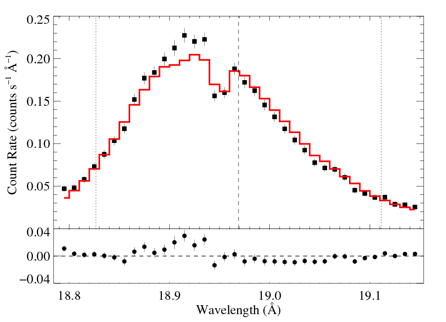
Isotropic porosity
Here we fit models with isotropic porosity (and still using the Rosseland bridging law), for the same set of fixed terminal porosity length values. When hinf is allowed to be free, a best-fit value of hinf = 1.7 is found, indicating the (iso-)porous models are favored, though this result is only very marginally statistically significant. We show this best-fit iso-porous model first, and then the three standard models with hinf = 0.5, 1, and 5.
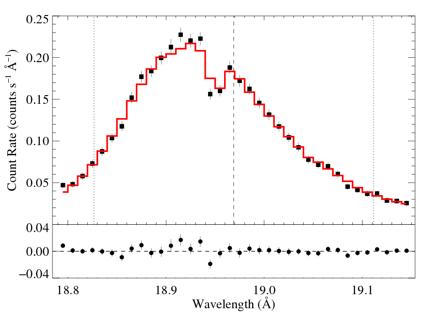
hinf free
|
[18.78:19.15]
vinf = 2250 β = 1 powerlaw continuum, n = 2; norm = 1.02e-3 q = 0 hinf = 1.71 +/- (0.81:2.54) taustar = 5.77 +/- (4.10:8.30) Ro = 1.55 +/- (1.42:1.64) norm = 4.67e-4 +/- (4.58e-4:4.75e-4) chisq = 171.08 for N = 72 |
Note that the iso-porous model is rather unconstrained by the Chandra data but the best-fit terminal porosity length is non-zero there, too.
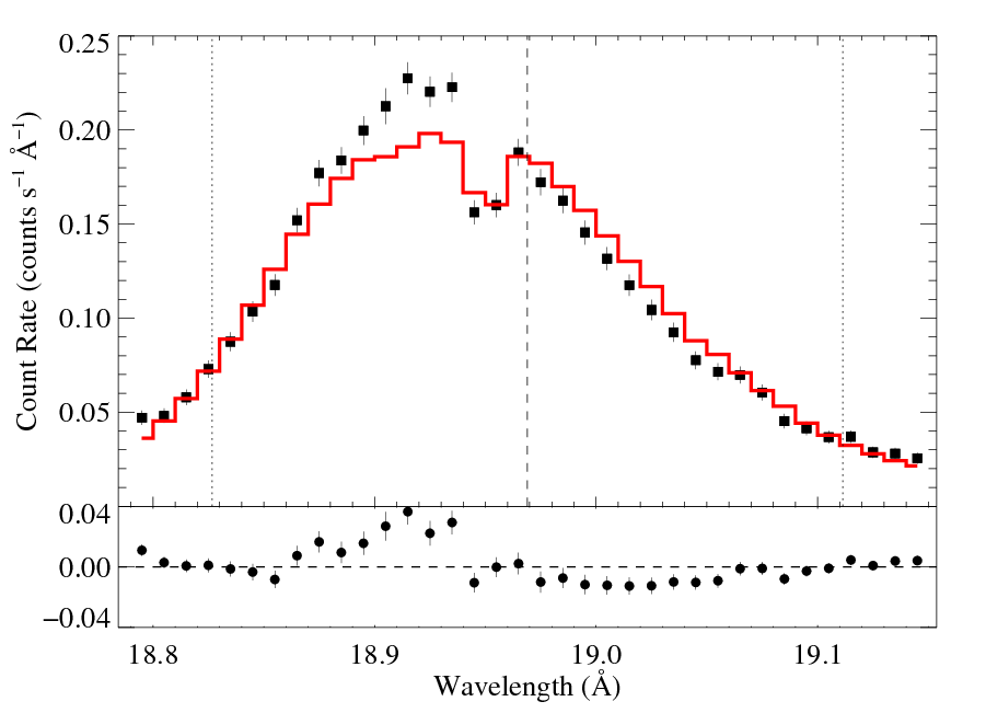
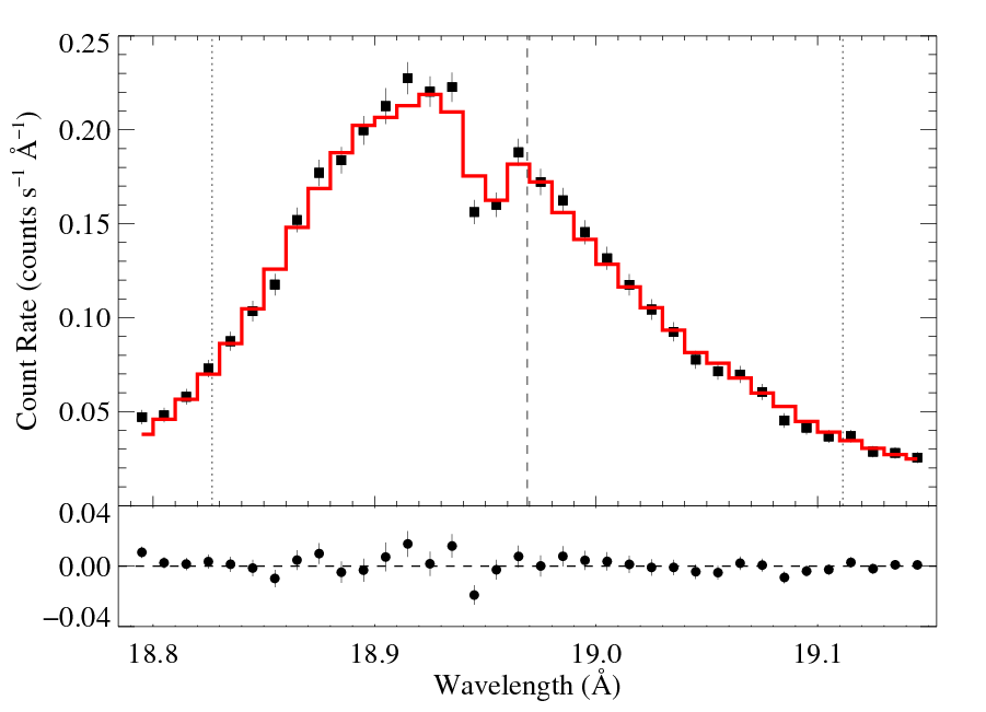
hinf = 0.5
|
[18.78:19.15]
vinf = 2250 β = 1 powerlaw continuum, n = 2; norm = 9.89e-4 q = 0 hinf = 0.5 (frozen) taustar = 3.70 +/- (3.55:4.15) Ro = 1.42 +/- (1.24:1.57) norm = 4.68e-4 +/- (4.59e-4:4.77e-4) chisq = 175.93 for N = 72 |
hinf = 1

|
[18.78:19.15]
vinf = 2250 β = 1 powerlaw continuum, n = 2; norm = 1.00e-3 q = 0 hinf = 1.0 (frozen) taustar = 4.42 +/- (3.94:4.98) Ro = 1.49 +/- (1.37:1.61) norm = 4.67e-4 +/- (4.58e-4:4.76e-4) chisq = 172.75 for N = 72 |
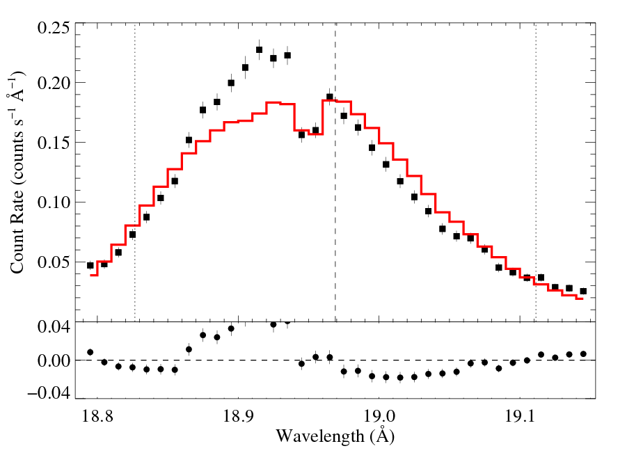
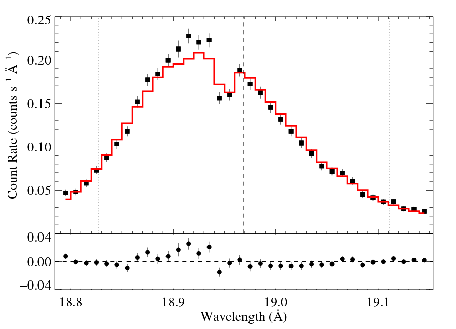
hinf = 5
|
[18.78:19.15]
vinf = 2250 β = 1 powerlaw continuum, n = 2; norm = 8.59e-4 q = 0 hinf = 5.0 (frozen) taustar = 20.03 +/- (17.3:23.8) Ro = 1.66 +/- (1.58:1.73) norm = 4.71e-4 +/- (4.62e-4:4.80e-4) chisq = 210.74 for N = 72 |
So, iso-porous models with modest porosity lengths provide good fits, but very large porosity lengths are ruled out. For porosity lengths of one or two stellar radii, the increase in taustar is at most a factor of two over the non-porous model.
Details of the fitting shown here for the O VIII line can be seen in gory detail in these xspec logs.
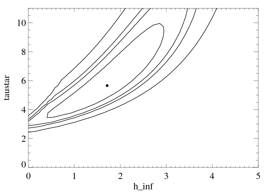
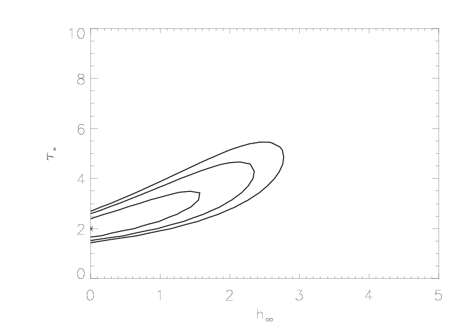
Confidence limits in taustar-hinf parameter space
|
Same contours as above for the Fe XVII line (except the re-scaling is slightly different, as the best-fit reduced chi square for this line is 2.7, rather than 2.3). Note the best-fit global model at hinf = 1.7.
Here too, there is good agreement with the corresponding Chandra result.
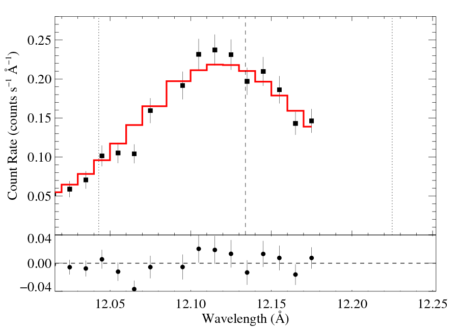
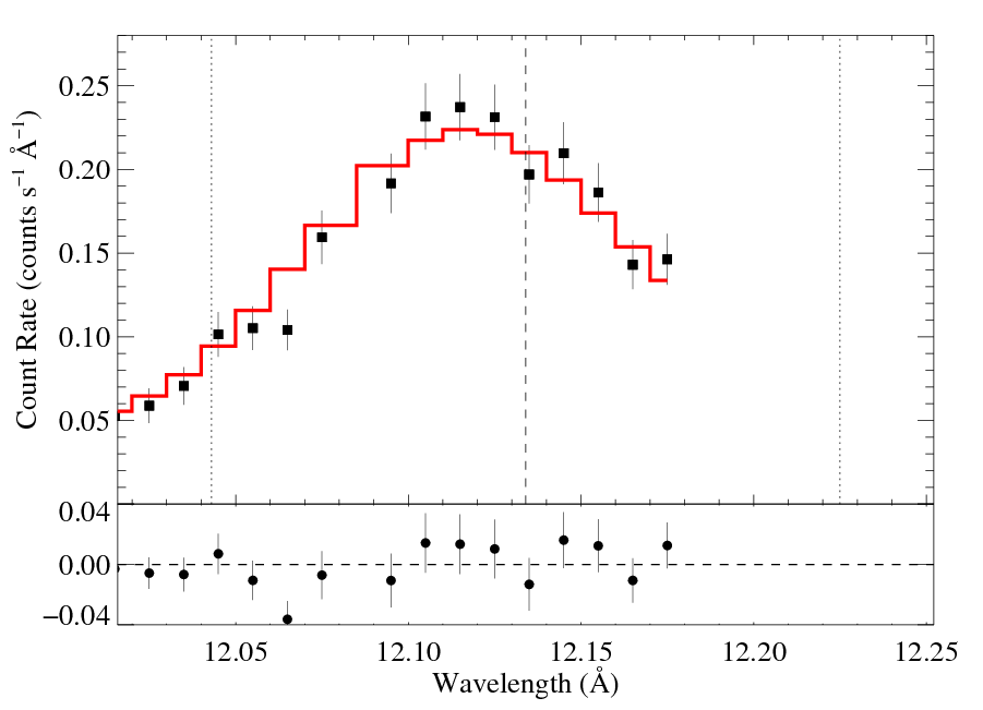
12.134 Angstroms: Ne X
Non-porous

|
[11.98:12.18]
vinf = 2250 β = 1 powerlaw continuum, n = 2; norm = 1.50e-3 q = 0 hinf = 0 taustar = 1.87 +/- (1.63:2.30) Ro = 1.46 +/- (1.01:1.63) norm = 3.07e-4 +/- (2.99e-4:3.15e-4) chisq = 49.27 for N = 37 |
Note that the reduced chi square isn't that bad -- 1.49; for only a 96.6% rejection probability. (This is due to lower signal-to-noise in this line.) So, we can formally use the chi square statistic, and confidence limits on single parameters correspond to Delta chi square = 1, as is usual. The exception is the extreme porosity fits, where the fit quality is poor enough that the use of the goodness of fit statistic to put constraints on model parameters is questionable.
Compare these results to the analogous model fit to the same line in the Chandra spectrum. There is very good agreement.
Anisotropic porosity
When the porosity length is treated as a free parameter, hinf=0 was preferred, with the non-porous fit parameters recovered (i.e. the data do not favor porosity). Below, we test several values of hinf, using anisotropic porosity, as we did, above.
hinf = 0.5
|
[11.98:12.18]
vinf = 2250 β = 1 powerlaw continuum, n = 2; norm = 1.18e-3 q = 0 hinf = 0.5 (fixed) taustar = 3.75 +/- (3.14:4.46) Ro = 1.35 +/- (1.18:1.52) norm = 3.17e-4 +/- (3.08e-4:3.25e-4) chisq = 55.86 for N = 37 |
hinf = 1
|
[11.98:12.18]
vinf = 2250 β = 1 powerlaw continuum, n = 2; norm = 9.97e-4 q = 0 hinf = 1.0 (fixed) taustar = 5.71 +/- (4.71:6.94) Ro = 1.41 +/- (1.27:1.56) norm = 3.22e-4 +/- (3.13e-4:3.30e-4) chisq = 64.79 for N = 37 |
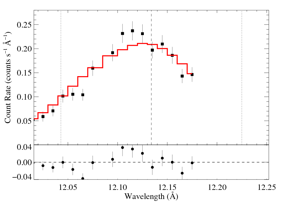
hinf = 5
|
[11.98:12.18]
vinf = 2250 β = 1 powerlaw continuum, n = 2; norm = 2.30e-4 q = 0 hinf = 5.0 (fixed) taustar = 63.99 Ro = 1.34 norm = 3.42e-4 chisq = 101.31 for N = 37 |
So, the anisotropic porosity models provide poor fits when the terminal porosity lengths are large.
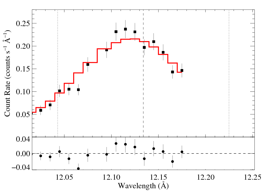
Isotropic porosity
When hinf is allowed to be free, a best-fit value of hinf = 0 is found, indicating that non-porous models are favored.
hinf = 0.5
|
[11.98:12.18]
vinf = 2250 β = 1 powerlaw continuum, n = 2; norm = 1.49e-3 q = 0 hinf = 0.5 (fixed) taustar = 2.17 +/- (1.88:2.61) Ro = 1.48 +/- (1.29:1.64) norm = 3.07e-4 +/- (2.99e-4:3.16e-4) chisq = 49.37 for N = 37 |
hinf = 1

|
[11.98:12.18]
vinf = 2250 β = 1 powerlaw continuum, n = 2; norm = 1.45e-3 q = 0 hinf = 1.0 (fixed) taustar = 2.56 +/- (2.18:3.13) Ro = 1.50 +/- (1.34:1.64) norm = 3.08e-4 +/- (3.00e-4:3.16e-4) chisq = 49.51 for N = 37 |
hinf = 5

|
[11.98:12.18]
vinf = 2250 β = 1 powerlaw continuum, n = 2; norm = 1.31e-3 q = 0 hinf = 5.0 (fixed) taustar = 14.10 +/- (9.80:20.79) Ro = 1.53 +/- (1.42:1.65) norm = 3.15e-4 +/- (3.07e-4:3.23e-4) chisq = 53.75 for N = 37 |
So, iso-porous models provide good fits, but very large porosity lengths require models with very high taustar.
Details of the fitting shown here for the Ne X line can be seen in gory detail in these xspec logs.
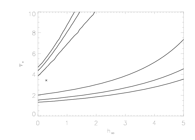
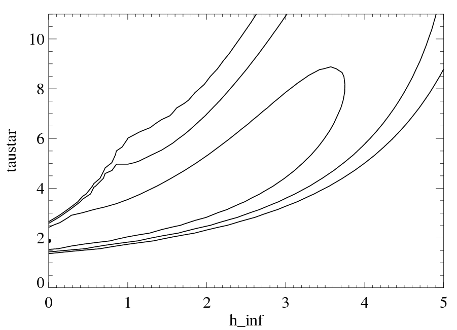
Confidence limits in taustar-hinf parameter space
|
Here too, there is good agreement with the corresponding Chandra result, although the RGS data doesn't provide as good constraints as the Chandra does.
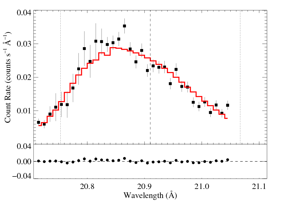
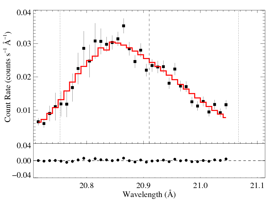
20.910 Angstroms: N VII
Non-porous

|
[20.70:21.05]
vinf = 2250 β = 1 powerlaw continuum, n = 2; norm = 6.99e-4 q = 0 hinf = 0 taustar = 5.19 +/- (3.95:6.15) Ro = 1.47 +/- (1.01:2.16) norm = 1.71e-4 +/- (1.58e-4:1.80e-4) chisq = 37.46 for N = 34 |
The fit is formally good, because the signal-to-noise is relatively low, and the errors are primarily statistical. Note the quite high taustar (albeit with large errors). This is consistent with the higher opacity model in Fig. 14 of Cohen et al. 2010. That higher opacity model assumes nitrogen enhancement.
Compare these results to the analogous model fit to the same line in the Chandra spectrum. There is pretty good agreement.
Anisotropic porosity
When the porosity length is treated as a free parameter, hinf=0 was preferred, with the non-porous fit parameters recovered (i.e. the data do not favor anisotropic porosity). Below, we test several values of hinf, using anisotropic porosity.
hinf = 0.5

|
[20.70:21.05]
vinf = 2250 β = 1 powerlaw continuum, n = 2; norm = 5.23e-4 q = 0 hinf = 0.5 (fixed) taustar = 8.38 +/- (6.20:11.20) Ro = 1.60 +/- (1.23:2.08) norm = 1.75e-4 +/- (1.63e-4:1.88e-4) chisq = 46.36 for N = 34 |
hinf = 1
|
[20.70:21.05]
vinf = 2250 β = 1 powerlaw continuum, n = 2; norm = 2.96e-4 q = 0 hinf = 1.0 (fixed) taustar = 14.44 +/- (10.80:19.82) Ro = 1.68 +/- (1.33:2.16) norm = 1.83e-4 +/- (1.69e-4:1.97e-4) chisq = 53.54 for N = 34 |
hinf = 5

|
[20.70:21.05]
vinf = 2250 β = 1 powerlaw continuum, n = 2; norm = 2.48e-11 q = 0 hinf = 5.0 (fixed) taustar = 100 Ro = 1.66 norm = 1.95e-4 chisq = 70.38 for N = 34 |
These anisotropic porosity models can be rejected, statistically. They don't look quite as bad as for some of the other lines because the signal-to-noise of this line is low.
Isotropic porosity
When hinf is allowed to be free, a best-fit value of hinf = 0.48 is found, but this model is statistically indistinguishable from the non-porous model. (And because it's so similar to our standard hinf = 0.5 case, we won't bother showing it here.)
hinf = 0.5

|
[20.70:21.05]
vinf = 2250 β = 1 powerlaw continuum, n = 2; norm = 7.30e-4 q = 0 hinf = 0.5 (fixed) taustar = 6.34 +/- (4.70:8.54) Ro = 1.72 +/- (1.15:2.22) norm = 1.70e-4 +/- (1.57e-4:1.82e-4) chisq = 37.28 for N = 37 |
hinf = 1

|
[20.70:21.05]
vinf = 2250 β = 1 powerlaw continuum, n = 2; norm = 7.48e-4 q = 0 hinf = 1.0 (fixed) taustar = 7.51 +/- (5.50:10.55) Ro = 1.86 +/- (1.46:2.30) norm = 1.70e-4 +/- (1.59e-4:1.82e-4) chisq = 37.37 for N = 37 |
hinf = 5
|
[20.70:21.05]
vinf = 2250 β = 1 powerlaw continuum, n = 2; norm = 6.02e-4 q = 0 hinf = 5.0 (fixed) taustar = 28.32 +/- (19.44:43.58) Ro = 2.12 +/- (1.82:2.52) norm = 1.75e-4 +/- (1.63e-4:1.86e-4) chisq = 41.86 for N = 37 |
Details of the fitting shown here for the Ne X line can be seen in gory detail in these xspec logs.
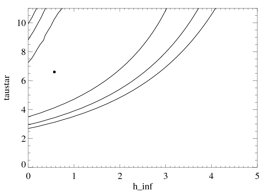
Confidence limits in taustar-hinf parameter space
|
The constraints are not severe, but as with the other lines, this figure shows that taustar increases rapidly beyond hinf values of about unity. It also shows that hinf is not well constrained, and the data are completely consistent with no porosity.
last modified: 16 December 2011