ζ Pup: tradeoff between porosity and mass-loss rate reduction as constrained by line-profile data
Here we examine the elements of the profile modeling, using the Fe XVII line at 15.014 A as a test-case, investigating the influences of various parameters and assumptions. We introduce two different porosity models and fit them to the Fe XVII line. We conclude with an analysis strategy that we use for the remainder of lines in the spectrum.
Skip right to the results page.
Baseline analysis (no porosity): Fe XVII at 15.014 Angstroms
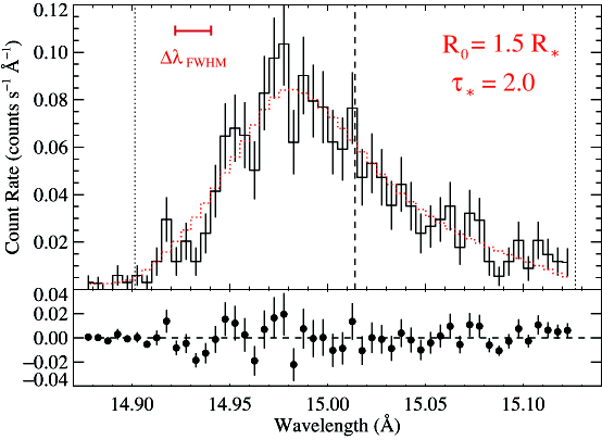
Here is the best-fit Owocki & Cohen (2001) model fit to one of the strongest, relatively unblended lines in the Chandra MEG spectrum (-1 and +1 orders coadded) of ζ Pup. Note that preliminary results appear in the Potsdam proceedings.
|
[14.87:15.13]
vinf=2250 β=1 powerlaw continuum, n=2; norm=1.91e-3 q=0 hinf=0 taustar=1.97 +/- (1.63:2.35) uo=0.655 +/- (0.605:0.725) norm=5.24e-4 +/- (5.04e-4:5.51e-4) rejection probability = 19% (C=95.11; N=102) |
Note: How to read the table of fit parameters.
Note: Where the uncertainties come from.
Exploring the effects of the continuum level
Notes on how the continuum level is determined and how sensitive the line fits are to the assumed continuum level.
Exploring the effects of the wavelength range
Comparison of the fit parameters for different choices of the wavelength range over which to fit the data.
Exploring the effects of the terminal velocity
Comparison of the derived fit parameters under different assumptions about the wind terminal velocity.
Exploring the effects of varying beta
Comparison of the derived fit parameters under different assumptions about the wind velocity law β value.
Exploring the effects of q - radially-dependent X-ray filling factor
Comparison of the baseline fit to one where q is a free parameter.
Exploring the effects of background subtraction
Comparison of the fit results for background-subtracted and non-background-subtracted data. Although we subtracted the background in all the fitting experiments to the Fe XVII line at 15.014, we will not subtract the background when we analyze high S/N lines in general.
Exploring the effects of including the HEG data in the fit
Comparison of the fit to the HEG data, and then a fit to the combined data. And a comparison of MEG and HEG for an isoporosity fit. It looks like including the HEG data in the fits to at least some of the lines will improve the derived constraints. Here is a large plot showing the portion of the HEG spectrum that has significant line emisison.
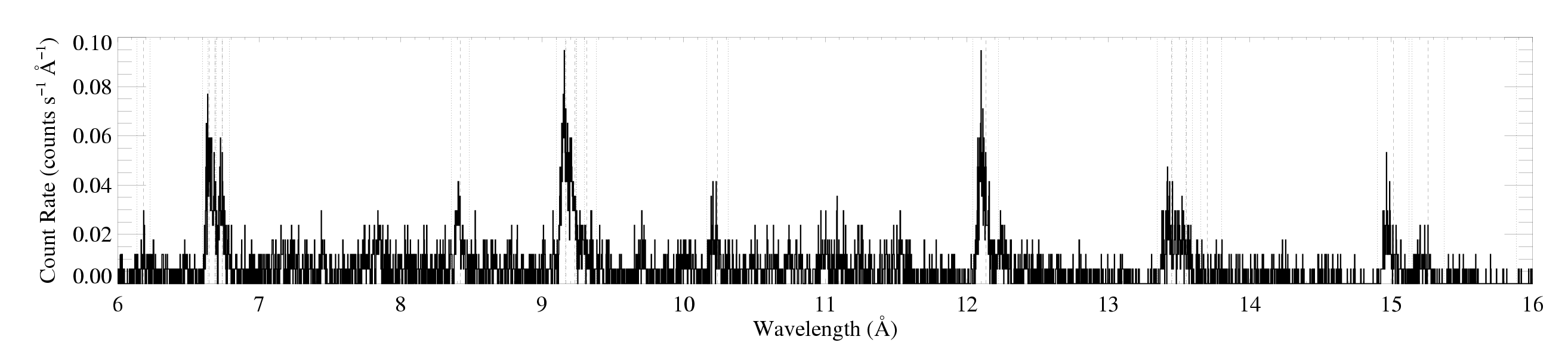
Preliminary conclusions
...about the sensitivity of the fitting results to the parameters and effects discussed above are summarized. Ultimately, we can go with a standard procedure, including using beta=1, and the Rosseland bridging law for isoporosity, that are based on efficient computation. But we can show how the results vary for one or two lines when we use beta=0.8, for example, and/or the exponential opacity bridging law, and use this variation as a guide to the magnitude of systematic errors in our analysis.
Isotropic (spherical clumps) porosity model (Owocki & Cohen, 2006): Fe XVII at 15.014 Angstroms
Best-fit model and confidence limits on the model parameters are summarized. Note that we also explore the effects of the different bridging laws in the context of isoporous models. And plot a small suite of porous profile models (Fig. 4 in the Potsdam proceedings).
Anisotropic (pancakes) porosity model: Fe XVII at 15.014 Angstroms
Best-fit model and confidence limits on the model parameters are summarized. Here we also explore the effects of the different bridging laws
Analysis strategy
Given the results for the 15.014 line, here is a basic strategy for analyzing the rest of the data, in which we balance clarity and efficiency on the one hand and thoroughness and a realistic assessment of (systematic as well as statistical) uncertainties on the other.
Results from fitting the rest of the lines in the spectrum.
last modified: 5 August 2008