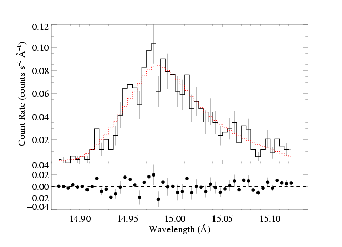
Fe XVII 15.014 Angstroms
Models with isotropic porosity - clumps shaped like spheres
We look only at the MEG data in this exercise, but at the bottom of this page we link to a new sub-page that explores the effects of including the HEG data in the isoporosity modeling.
|
[14.87:15.13]
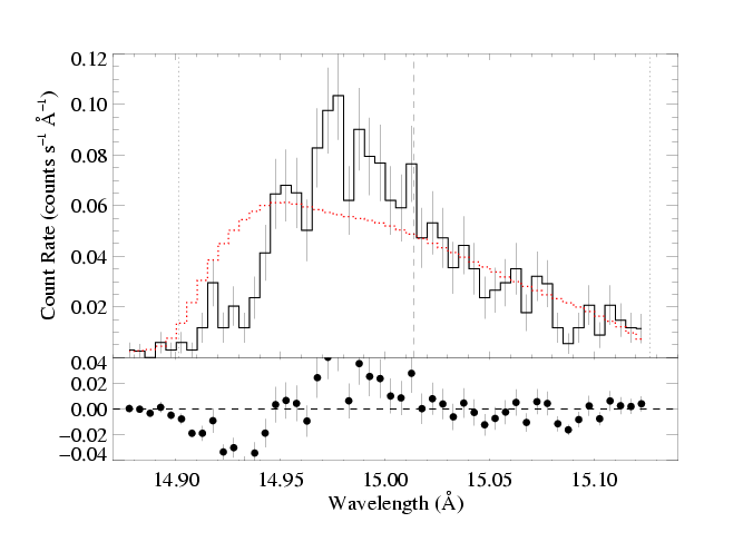
vinf=2250 β=1 powerlaw continuum, n=2; norm=1.91e-3 q=0 hinf=0.00 +/- (0.00:0.66) and for 90% confidence, (0.00:1.49) taustar=1.97 +/- (1.65:2.54) uo=0.655 +/- (0.605:0.720) norm=5.27e-4 +/- (5.04e-4:5.50e-4) rejection probability = 23% (C=95.09; N=102) |
Note that the best-fit hinf=0, so the other best-fit parameters are (nearly) identical to the original (baseline - shown at the top of the background page) model fit where hinf was held constant at zero. However, note also that some of the uncertainty ranges are bigger, because non-zero values of hinf are allowed when the confidence grid is calculated. Specifically, somewhat larger values of taustar are allowed because finite values of the porosity length reduce the effective wind opacity (allowing for larger atomic opacity based optical depths; larger taustar values, in other words - this is the trade-off that we are primarily studying in this work).
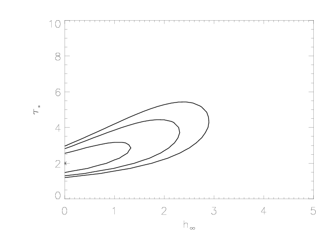
Below, we examine the joint constraints on taustar and hinf. Note that the confidence limits extend to larger values of the terminal porosity length when its distribution is considered jointly with that of taustar:
Here are the joint constraints on taustar and uo:
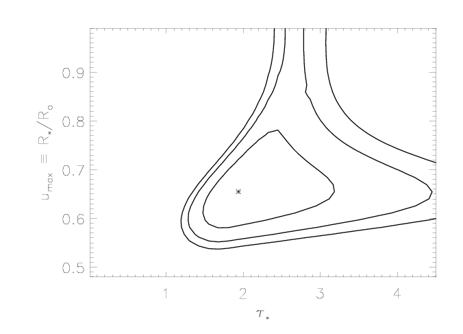
Note that the extent of the taustar confidence limits - at the high end - has expanded, now that we're allowing for porosity (letting hinf be a free parameter). Compare the confidence limit contour plot above to the one we show on the uncertainties page, also in taustar-uo space but without any porosity (hinf=0):
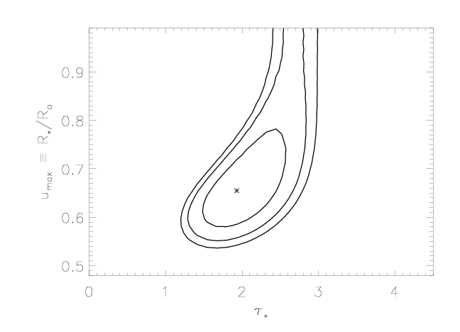
Comparing these two plots, we see that allowing for porosity enables models with higher taustar values to fit the data adequately; and looking at the first confidence limit plot, in taustar-hinf space, we can see explicitly what the trade-off is between these two parameters.
The above constraints get somewhat tighter when the HEG data are included.
We might now investigate the extent to which porosity can explain the profile shape in the context of higher mass-loss rates. Specifically, if the literature mass-loss rate is correct, then (a) can porosity explain the relatively symmetric profile (as well as a reduction in mass-loss rate in the context of a non-porous wind can) and (b) what levels of porosity (what values of hinf) are required?
To investigate this, and to demonstrate (again; we've already shown that taustar is low and has tight constraints) that a non-porous profile model with a high taustar (consistent with the literature mass-loss rate) cannot fit the data, here is the best-fit (normalization and uo are free parameters) non-porous model with taustar=8 held fixed.
|
[14.87:15.13]
vinf=2250 β=1 powerlaw continuum, n=2; norm=1.91e-3 q=0 hinf=0 taustar=8 uo=0.98 +/- (basically unconstrained) norm=5.40e-4 +/- (constraints not meaningful) rejection probability = 100% (C=174.86; N=102) |
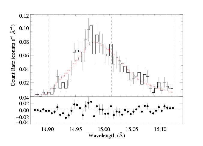
Clearly the fit is poor. Something is needed. In the fits shown above - the baseline fit - we show that reducing the fiducial optical depth, taustar, by a factor of four leads to a good fit. Below, we show that a decent fit can be achieved even with taustar=8 if we introduce (isotropic) porosity.
|
[14.87:15.13]
vinf=2250 β=1 powerlaw continuum, n=2; norm=1.91e-3 q=0 hinf=3.37 +/- (2.58:4.23) and for 90% confidence, (2.21:4.95) taustar=8 uo=0.638 +/- (0.603:0.685) norm=5.30e-4 +/- (5.05e-4:5.52e-4) rejection probability = 44% (C=104.61; N=102) |
Compare this fit and these constraints to those derived from the combined MEG and HEG data.
Note that the rejection probability is not very high. In other words, taken in isolation this is not a bad fit. However, ΔC=9.5 compared to the best-fit model where taustar and hinf are both free (the global best-fit model with isotropic porosity shown at the top of this subpage which is effectively identical to the baseline model fit since the best fit porosity length is zero). A value of ΔC=9.5 for one parameter of interest implies significance of >99% in terms of preferring one model over the other. In other words, the non-porous, low taustar model is preferred with >99% confidence over the high taustar, high porosity length model.
Here are the two models overplotted with the data: the red model is the global best fit, with taustar=2.0 and hinf=0.0, while the blue model is the best-fit in which taustar is held fixed at a value consistent with the literature mass-loss rate, taustar=8, and the best-fit value of hinf=3.37.
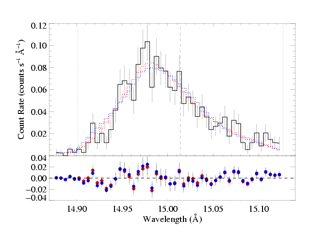
The differences are not great - and as we've already pointed out, the porous model cannot be rejected as a "bad fit" - however, there are systematic differences between the two models (note especially the bulge on the blue wing in the porous model), and from a formal statistical point of view, the non-porous (red) model is preferred over the high optical depth, high porosity (blue) model with a high degree of significance. To more clearly show the systematic differences between these two models, and generally between porous and non-porous profile morphologies, we also show these two models at infinite resolution and without the data (and for good measure, throw in the non-porous, high taustar model too):
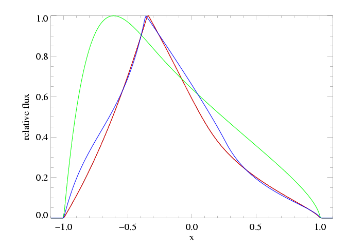
Here the best-fit global model is shown in red, while the model with taustar=8 frozen and a free porosity length (with a best-fit value of hinf=3.37) is shown in blue. The green model is taustar=8, hinf=0.
Finally, we can compare the confidence limits on our two types of models (tuastar free and thus generally preferring low values, and taustar = 8 fixed, to impose the conditions implied by the literature mass-loss rate; i.e. the blue and red models in the two above plots) in the two-dimensional parmeter space of our confidence limit contour plots:
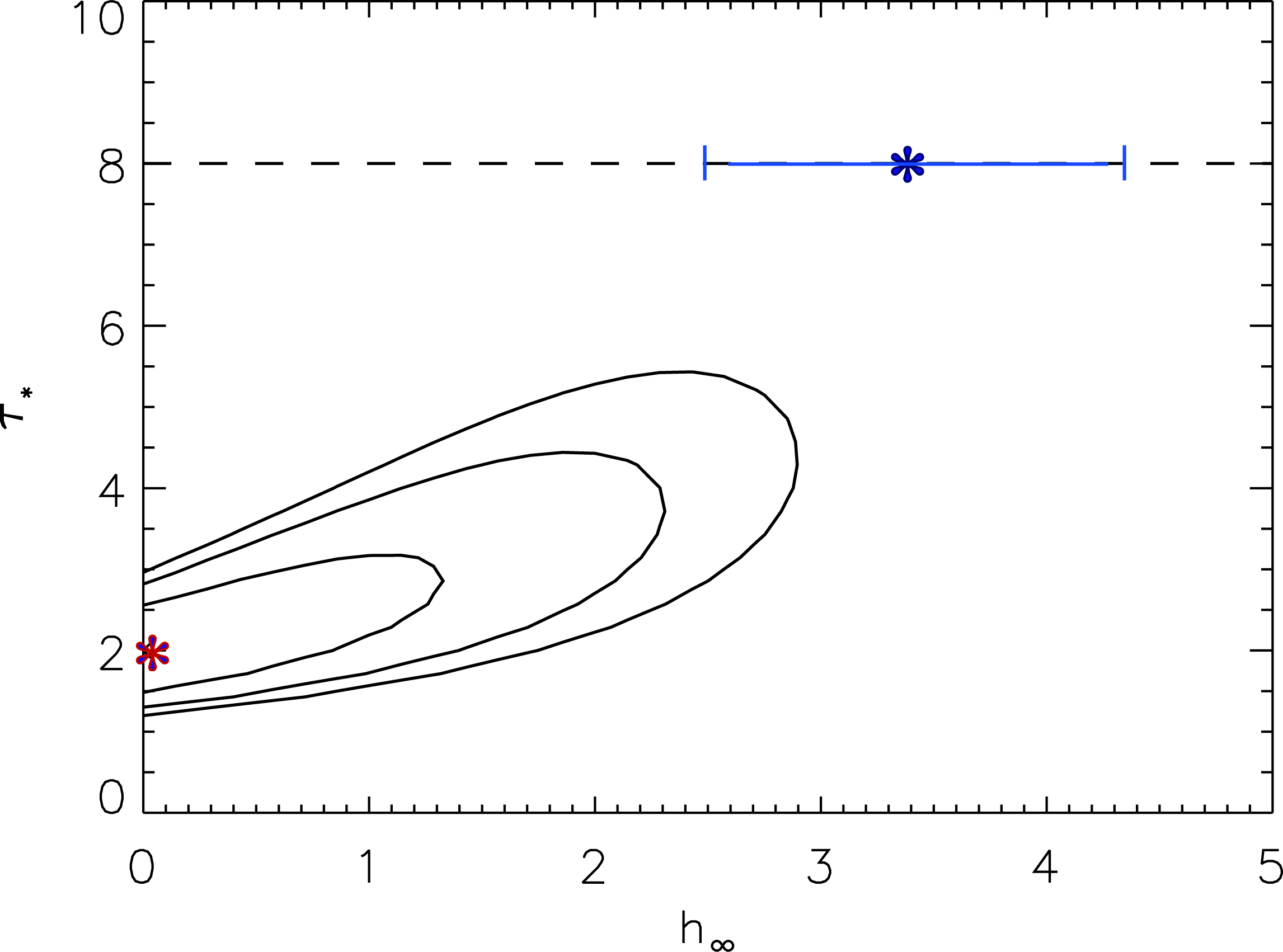
The red asterisk represents the global best-fit model, in which the porosity length is zero, while the blue asterisk represents the best-fit model where taustar=8, the value implied by the literature mass-loss rate. Given taustar=8, the best-fit hinf=3.37, and the 68% confidence limits on hinf given taustar=8 are shown as the horizontal blue bar.
We have reproduced much of this analysis for the combined HEG and MEG data.
We explore the effects of the opacity bridging law.
Back to main page.
last modified: 16 July 2008