Astronomy 16: Modern Astrophysics
Archive of Assignments
Week 14
posted 12/9
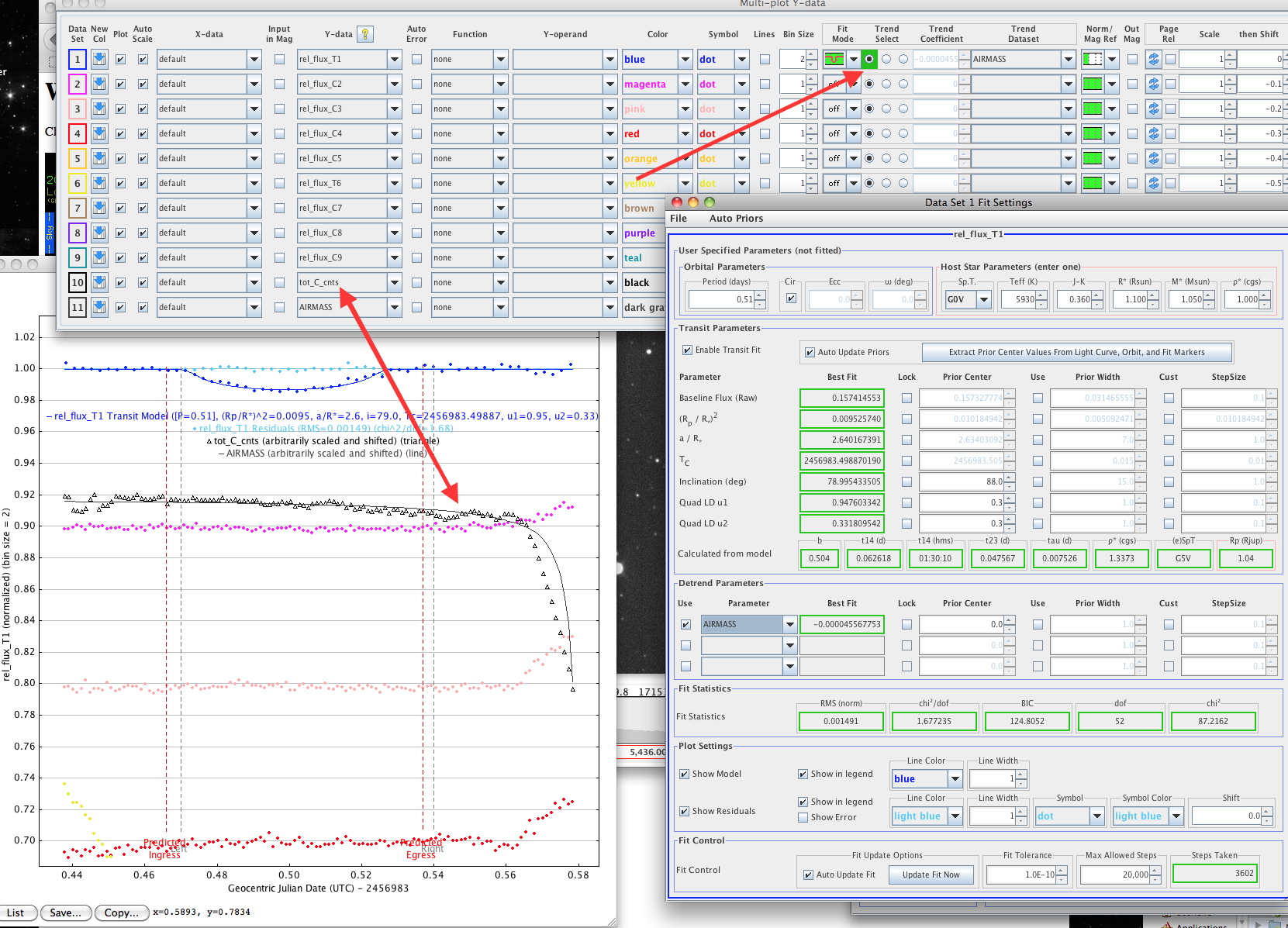
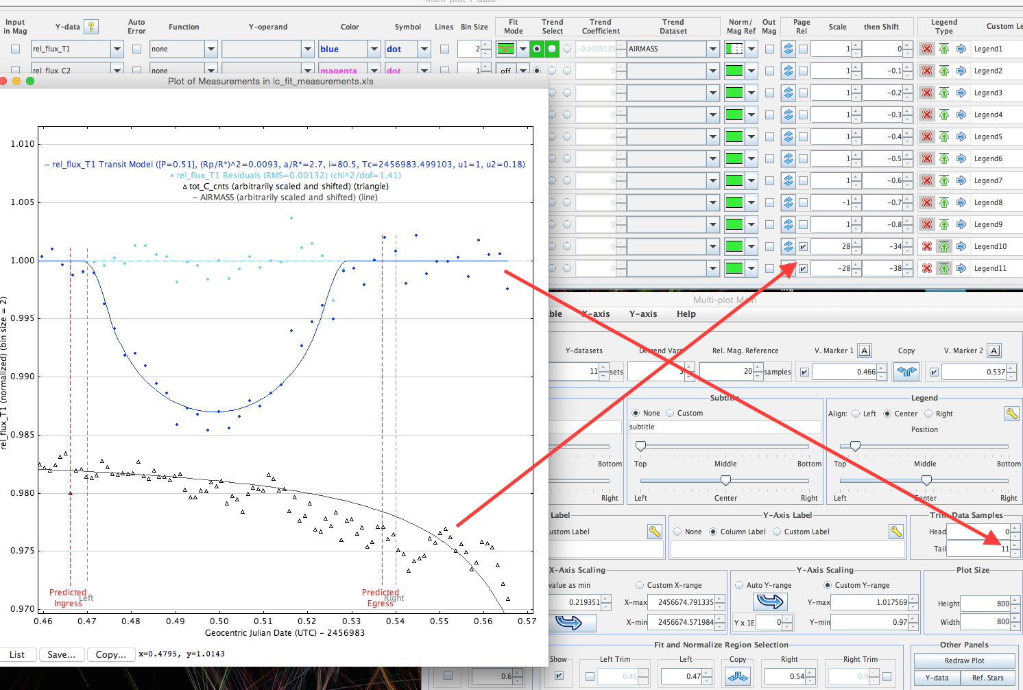
Take a look at these tips about the AIJ data analysis for lab 5 [pdf] (they're the same ones I emailed around 9pm). There are figures [1 and 2], too.
Look over the slides I showed in class on Tuesday [pdf].
posted 12/7
Please read these instructions for your lab work and write-up [pdf], and let me know if you have any questions. Note that the write-ups are due on Thursday, by 5pm.
posted 12/6
Please look over the reading assignment for Tuesday [pdf], do the reading, and come to class prepared to go over the material and ask questions.
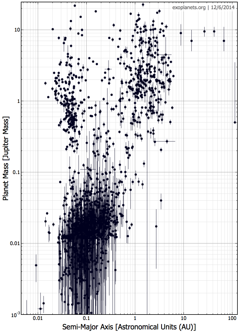
You can explore exoplanets.org and make your own customized plot of any number of different trends seen in the (currently known) 1499 exoplanets with good orbital determinations.
Week 12 - 13
posted 12/4
Look over the slides I showed in class on Thursday [pdf] on dark matter and flat galaxy rotation curves.
posted 12/2
Read over this background information on this week's lab [pdf] prior to coming to our lab meeting on Wednesday night.
Look over the exoplanet slides I showed in class on Tuesday [pdf] and your notes and Ch. 12 prior to coming to our lab meeting on Wednesday night.
posted 11/30
Please carefully look over this reading assignment, including the short list of topics to focus on [pdf] sometime on Monday. We'll discuss exoplanets on Tuesday and the Milky Way on Thursday. The exoplanet material will be useful for Wednesday night's lab, too.
Please finish up your work for the WASP-11 lab. We'll be analyzing data I just took of an exoplanet candidate host star for our next lab. I'll send out data and some instructions by Tuesday. Note that I have office hours on both Monday and Tuesday afternoon.
posted 11/25
Our next homework assignment, homework #7 [pdf] is due on Wednesday, December 3.
We will have a lab meeting on Wednesday night, December 3. Stay tuned for both feedback on your WASP-11 light curves and information about the next, and final, lab meeting.
A more detailed reading assignment will be posted shortly, but most of Tuesday's class will be on exoplanets, and so you should read Ch. 12 (focusing mostly on sections 3 and 4, but sections 1 and 2 do provide some interesting context with respect to the planets in our own solar system).
Week 11
posted 11/19
Here's a reading assignment/topic-summary for this and next week.
posted 11/16
You should study for Tuesday's midterm. Read these guidelines and let me know if you have any questions. New: There will not be any questions on the material from Ch. 6 (telescopes/observational astronomy).
posted 11/13 (posted last week)
By Monday (but talk to me if you can't) you should go through the tutorial on photometry and lightcurve making, and produce a light curve for WASP-11, and email it to me.
Week 10
posted 11/14
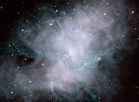
Take a look at images from Thursday's class. The expanding Crab Nebula gif is linked from the image below:
posted 11/13
By Monday (but talk to me if you can't) you should go through the tutorial on photometry and lightcurve making, and produce a light curve for WASP-11, and email it to me.
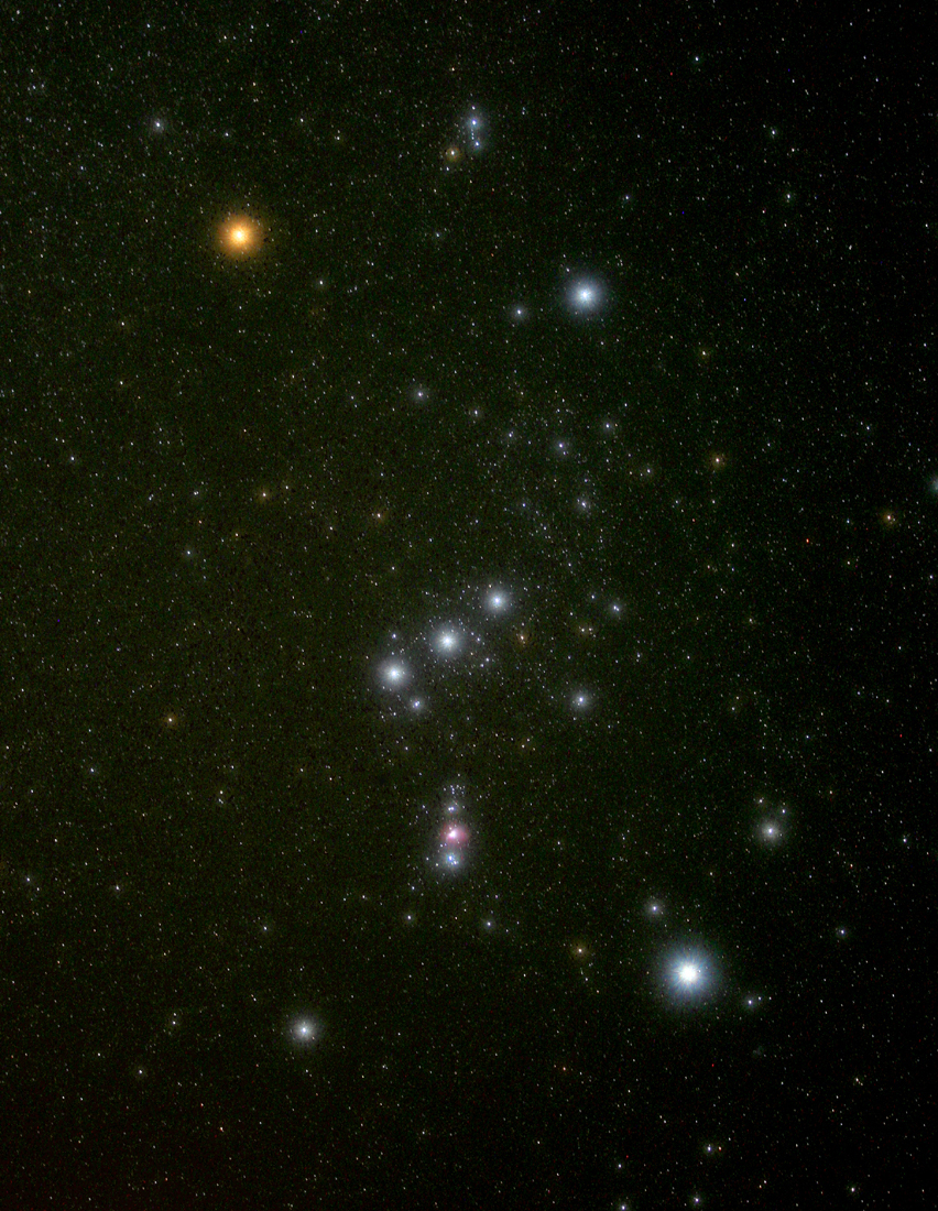
Take a look at these images from Tuesday's class: Gas and dust in Orion from APOD; A numerical simulation of collapsing molecular cloud complex, from this German research group's page on molecular clouds; And star formation on a galactic scale which includes that picture of Orion with the molecular gas superimposed. Also, the protostellar accretion disk with gaps where...planets may be forming. That image was taken with the new Chilean radio telescope array, the Atacama Large Millimeter Array (ALMA).
posted 11/12
Look over the reading assignment for this week. It includes the Ch. 6 material for the lab that's been posted below, as well as material on stellar remnants for Thursday's class.
posted 11/9
The objects I observed for you are available on this server. Before coming to lab on Wednesday, reduce your data and make a three- or four-color composite image. The data reduction and image compositing instructions that you received before our first lab are now linked on the right side of this page (as well as in the archive of old assignments). As you choose colors for your image slices, you might want to consult the filter response plots on the second-to-last page of the instructions. Two more things: (1) You should be careful evaluating and reducing your data – check each image and throw bad ones out, make sure reduction steps and alignments really worked right, be very careful when choosing input files, and if your final images look bad, go back and figure out what went wrong and fix it. And, (2) when doing the final step of combining your single-color images into a composite image, I've found that if you keep the menu setting to "composite" you can step through each slice and adjust the grayscale (brightness/darkness) for each one in sequence without your new settings being forgotten. Once you've reset them, going back and changing any one of them again first sets the grayscale levels back to their original settings. Get in touch if you want some help with this, or any other, step (before coming to lab on Wednesday). You should email me your final image of your object before our lab meeting.
I will give you some data to put on your computer, and some information about exoplanet transits and their light curves, soon. I'll expect you to read this information and also some of Ch. 6 (see below) before coming to lab as well. I will email you when it's available.
Reading for this week will be a little different. On Tuesday, we are going to discuss stellar evolution and also pulsation. So, material from Ch. 17, which you've already read. I'll post a new reading assignment (focused on Ch. 18: Stellar Remnants) soon, but that material won't be covered till Thursday. Instead, you should spend the beginning of your week reviewing the stellar evolution and pulsation material from the textbook, and preparing for lab. That should include rereading the first section of Ch. 6: Astronomical Detection of Light (I assigned it to you a few weeks ago, before our last lab meeting). Skim Secs. 2 and 3 (but read the figures and their captions carefully). Read Secs. 4 and 5 and skim Sec. 6.
Week 9
posted 11/7
Please look at the slides I showed in class on Tuesday [pdf] (there are also a few from the previous class, showing binary star spectra). You should be able to explain everything in those slides, and answer the questions that are on a few of them.
posted 11/4
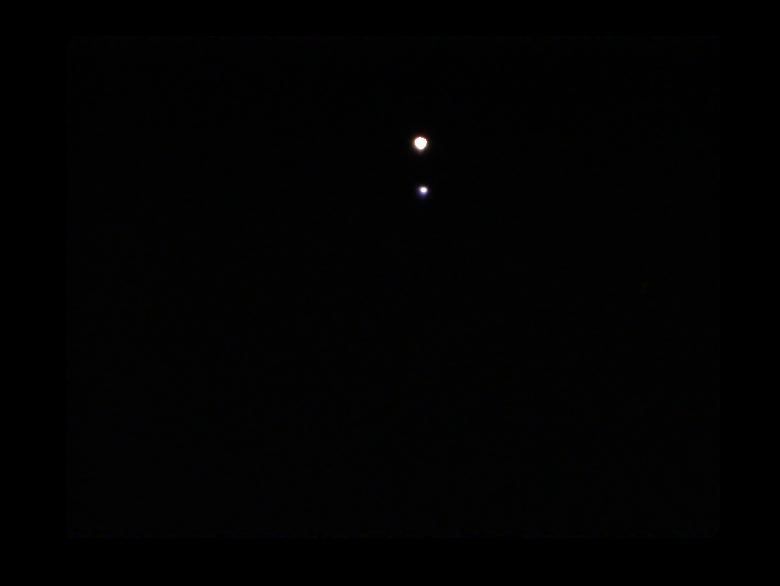
You can read a little more about Albireo. And look at the image taken by Astro 16 students in 2009.
posted 11/3
Our sixth homework assignment is now available. It's due on Wednesday, November 12, at 11 AM. You have a lot of time to do this homework, but the assignment is longer than usual. You should look over the problems soon, even if you don't have time to start it right away.
posted 11/1
In preparation for Tuesday's class, spend a few minutes building binary systems and seeing how their properties affect their observables: eclipsing binaries and their light curves and spectroscopic binaries and their radial velocity curves. You will need a working version of Java on your computer to use that second one.
The reading assignment for the week is now available. Binary star wrap-up and star formation and stellar evolution (Ch. 17).
Week 8
posted 10/29
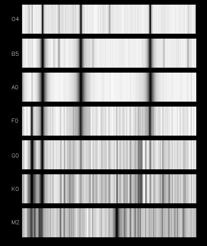
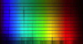
In preparation for (and follow-up after) Thursday's class, spend a few minutes building binary systems and seeing how their properties affect their observables: eclipsing binaries and their light curves; spectroscopic binaries and their radial velocity curves. You will need a working version of Java on your computer to use that second one. Also, take a look at these examples of stellar spectra of different spectral types and also look at these detailed stellar spectra, comparing zoomed in portions of the Sun's spectrum to the spectrum of the hotter star, Vega. Finally, here are quite a few examples of real stellar spectra that cover most of the full visible range. Can you see the extent to which these spectra resemble blackbodies and the ways in which they deviate from a perfect Planck function?
posted 10/26
A shorter-than-usual reading assignment for the week is now available. Binary stars and stellar masses is the new stuff, but the HR diagram and the magnitude system, already assigned last week, is what we'll spend most of Tuesday's class on.
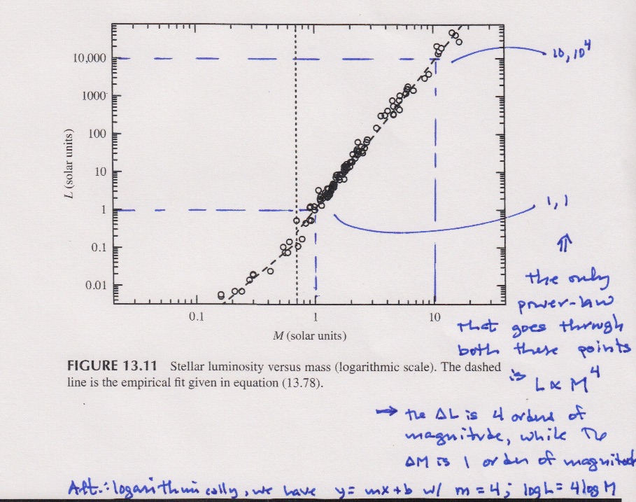
Also, take a look at this annotation of Fig. 13.11 - the mass-luminosity relationship, which we looked at in class on Thursday, and from which we fit a power-law with index 4. If you want to reinforce your understanding of how that's done, have a look at mine. And take another look at the spectral type sequence, including the description underneath the image and look back over the corresponding information in the textbook (Sec. 14.2).
posted 10/25
Our fifth homework assignment is partially available. Two more problems will soon be added. It's due on Tuesday, October 28, at the beginning of class. Update 10/26 The full assignment includes two additional problems, on the magnitude system, which was in last week's assigned reading, and which we'll go over in class on Tuesday.
Following up on our lab meeting last week, you should each send me the name of an object you'd like to observe, as well as an airmass plot for it and an annotated finding chart. Here are the resources I've posted over the last week or two: this short article with many pictures about M17; the airmass plotter (the airmass is the cosecant of an object's altitude); and the tool for making finding charts.
Week 7
posted 10/14
Our fourth homework assignment is quite short. It's due on Wednesday, October 22.
posted 10/15
Take a look at the reading assignment for next week's classes.
We'll be doing some more data reduction and image manipulation on Wednesday in lab. You can start thinking about what object you'd like to observe. Take a look at this short article with many pictures about M17, a giant star formation region. The "M" designation means the object is in the Messier Catalog of fuzzy objects that might be mistaken for a comet by an 18th Century astronomer. There are links to articles about other Messier objects at the bottom of the article.
Note that you can start to see some of the concepts we've been discussing in a more abstract, physics context in class come into play in the article. Massive stars with short lifetimes because of their very high luminosities, for example. And note also that at the end of the article a multiwavelength view of M17 is given. There is a strong X-ray source in the nebula, which the author says could be an accreting black hole or a background quasar. But I'm actually working on a paper now showing that it's a quadruple system of four massive stars (two pairs of binaries that are themselves orbiting each other) and that the strong X-ray emission comes from interactions between the powerful winds of each binary pair.
Also: The images in the article are beautiful! Ours won't be as good. And we can't observe this object anyway, as it's setting soon after sunset. If you want to see how observable a given object might be, you can use the Tapir software written by Eric Jensen - try the airmass plots (the airmass is the cosecant of an object's altitude). And also try making a finding chart. Take a look at some of the Messier objects and think about which one you'd like to observe.
Finally, the Stellarium software the author uses to make plots of the sky is freely available (see the link on the right side of this page).
While reading a few of the Messier posts, I came across this post debunking a "cold fusion" device. It's quite brief, but touches on much of the same physics as our discussion of nuclear reactions last Thursday. It even has the plot of nuclear binding energy vs. atomic mass that I drew on the blackboard. Take a look.
Week 6
posted 10/9
Play around with this gravity simulator. Note how if you set up any array of masses, they'll all collapse into a single large mass. To get orbits, you need to give some objects (tangential) velocity.
Planet Crash is another simulator/game. You have to start with circular orbits, but it has other interesting features.
posted 10/6
You should read the reading assignment for week six. Note that for Tuesday, it's just review of material that was assigned last week. But DO review it; read the assignment itself even if you don't have time to go back to the textbook before Tuesday's class. For Thursday, it's nuclear reactions to wrap up Ch. 15. There, too, read the assignment itself, especially the new questions/notes, before coming to class on Thursday, even if you don't have time to thoroughly read the textbook. I still think it's important to read the assigned textbook material before coming to class, but I acknowledge that studying for the midterm will likely take priority.
posted 10/4
The midterm will be calibrated for 75 minutes, but you'll have two hours to complete it on Wednesday night. It will be closed book, and cover all the material I've assigned through the end of Ch. 5. So, up to the middle of Thursday's class. No hydrostatic equilibrium on the exam. The exam will be closed book. You'll be given copies of the two tables from the Appendix that are posted on the right side of this page. And, you'll be allowed to put together and bring to the exam with you one 8 1/2 by 11 piece of paper with your own hand-written notes. So, any equations you think you might need as well as any kind of notes you care to write - sketches, solutions for homework problems, etc. But it must be hand-written. You can write on both sides. And I'll collect your sheet of notes at the end of the exam. The exam will focus on basic concepts and their applications - no detailed applications of the Saha equation for example. But you should understand what the Saha equation is used for and how to use it. Equations that we talked about and used more in class (e.g. angle-size-distance, parallax, Kepler's third law) are more likely to show up on the exam. Some of the questions will involve calculations but others will require written responses (of a couple of sentences) and in some cases maybe sketches or diagrams.
A reading assignment for week 6 will be posted here shortly, but it will begin with reviewing the relevant parts of sec. 15.1 and 15.2 (assigned last week), and then moving on to the rest of Ch. 15.
Week 5
posted 9/28
Check out the reading assignment for week 5 [pdf]. Note that on Tuesday we'll still be covering the material from Ch. 5. By Thursday, we'll be on to hydrostatic equilibrium and beginning stellar structure. Read this assignment/guidelines carefully. They include some questions and comments about the material from sections 9.2 and 15.1 and 15.2, to help you guide your preparation.
posted 9/27
Our third homework assignment [pdf] is now available. All the questions are on material from Ch. 5. Note that the last (fifth) question involves some calculations and plotting as well as some interpretation. You should take a look at the assignment, and especially that problem, quite soon, even if you don't have time to start it right away. It is due this Friday at 2pm.
Week 4
posted 9/21
Take a look at these reading guidelines for week four [pdf]. Update 9/22 I have added some specific information about what concepts (and equations and figures) you should pay the most attention to as you read this material, so please do take a look at it before coming to class on Tuesday (and again on Thursday).
Week 3
posted 9/14
Take a look at these reading guidelines for this week [pdf]. There's some specific information about the Doppler shift in there, but otherwise, it's almost entirely review of last week's material. This week's light reading load should provide a great opportunity for you to make progress on the homework that's due on Wednesday!
Week 2
posted 9/11
If you're still working on your lab write-up, you should consult this revised version of the lab manual [pdf] I gave you on Wednesday night. It has some added information and explanation (e.g. how to find the file header information; what the three different kinds of calibration files are). You may want to consult the guide for reducing data and making composite color image [pdf or MS Word]
Our second homework is now available. Update 9/15: A revised version clarifies problem number 3. The homework is due Wednesday morning. There will be another SA session on Monday night, from 7:30 to 8:30 in SC 102.
posted 9/7
Read these guidelines [pdf] for preparing for class this week. Summary: Tuesday's class will mostly be the end of week 1's topics. The first three sections of Ch. 5 will be discussed in class on Thursday, with a start on sec. 5.1 toward the end of Tuesday's class.
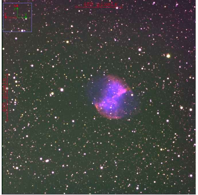
Our first lab meeting is this Wednesday night (8 to 11 pm, SC 187, no matter what the weather is like). You will be learning how to use the telescope (weather permitting) and learning how to reduce data from the telescope. I'd like you to get started working with some telescope data, so please go through this guide for reducing data and making composite color image [pdf] before coming to lab. You might prefer the MS Word version because then you can highlight embedded images and make them bigger if you're having trouble seeing all the information in them. You should budget a couple of hours to do this. You'll get so much more out of lab and be so much happier if you spend about that much time preparing. You should put the data on your own laptop if you've got one, and then bring it to lab on Wednesday night.
When you've finished going through the guide, you should have a nice color image of the Dumbbell Nebula (or M 27), like this:
posted 9/5
Our first homework assignment [pdf] is now available. It is short (four questions), covers material we've already discussed in class during the first week, and is due in class on Tuesday morning. Note that there will be an SA session on Monday night from 7:30 pm to 8:30 pm in SC 102.
posted 9/4
Review how the Greeks knew the size of the Moon, relative to the Earth, by noting its curved shadow on the Moon during a lunar eclipse and (estimated the ratio to be 3.7). Combining this with Eratosthenes's measurement of the Earth's circumference they could compute the actual size of the Moon (in meters, if they'd had them). And from that combined with the angular size of the Moon (about half a degree), they were able to compute the distance to the Moon. Make sure you understand and can explain (including the quantitative computations) how each of these steps was done.
In next Tuesday's class, we will begin with an application or two of the inverse square law. And then we'll discuss gravity, uniform circular motion, and orbits, as well as revisit Moon phases, and then see what questions you all have about the material from the week 1 assignment. By the end of Tuesday's class, we'll begin the material from the new (soon to be posted) assignment (update: posted 9/7).
Week 1
posted 8/30
The first thing to do to prepare for class is to study this website, including the four images at the top, and especially the class announcement, posted to the right, on the main page.
To prepare for the first class meeting, read this list of topics and reading assignments [pdf] for the first week. Give yourself a few days to do the preparation. As you'll see, I've provided you with some guidelines about what to focus on as you read. Please read this document carefully, and note that it is material for the entire first week, not just Tuesday's class. We'll cover the topics in more-or-less the order that they're listed, but by Thursday's class you should have completed all the preparation.
And to prepare for Tuesday's class and the course in general, go outside on at least two different evenings and find the crescent moon. Your goal is to track its motion and also its change in illumination. We'll discuss your observations in class, but you don't have to hand anything in.
The first homework assignment will be posted here shortly. It will be due on Wednesday, September 10 (probably; note the update (9/4)).
Return to the main class page.
This page is maintained by David Cohen
cohen -at- astro.swarthmore.edu
Last modified: December 13, 2014