Astronomy 6: Introductory Cosmology
Archive of Assignments
Week 12/14
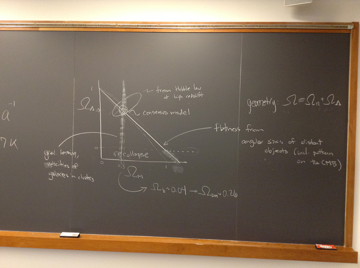
Update (Dec. 14): Look over my notes for our last class (Wed., Dec. 11), and also look over the summary sketch of the consensus model and how we know its parameters, from the blackboard on Wednesday.
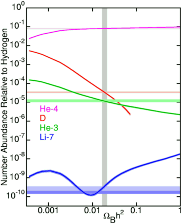
Also, look over this figure showing the predictions of the light element abundances based on the Big Bang Nucleosynthesis scenario, which I handed out and we discussed in class on Wednesday. Note that the free parameter of the model (plotted on the x-axis) is proportional to Omega_baryon. The higher the baryon density, the more reactions occur and, for example, the more helium gets produced. One key take-away from this figure is that all the light element abundances are predicted by the same Omega_baryon parameter value range. And that that value, about 0.04, is much lower than dynamical measurements of mass, which include both baryonic and non-baryonic dark matter.
Finally, check out one of the many cosmological model calculators available on the web. Or this one.
Update (Dec. 9): For our last class, on Wednesday, please read the rest of Ch. 24 (secs. 3 and 4), and read this one page article by Jim Holt that addresses the question of how we should think about the "fine tuning" of the Universe and how seriously we should take the idea of multiple universes. Also please listen to the TED talk by Sean Carroll on the early universe, entropy, and the arrow of time if you haven't done so already.
Update (Dec. 8): There is part of a new homework assignment available, on modeling the universe including the horizon distance and on the accelerating expansion. dark matter. It is due Thursday by noon. Note that what is posted as of Sunday afternoon is updated compared to what I emailed out earlier in the weekend but also that I'll be adding at least one more problem to the assignment soon.
For our next class meeting (Monday, December 9), please review sec. 24.2 and especially Figs. 24.6 and 24.7. Also: read this short article about the accelerating universe and dark energy.
Week 13
Update (Dec. 1): There is a new homework assignment on dark matter. It is due Wednesday by 10 am. This homework is designed to get you ready for our discussion of dark matter and the Bullet Cluster ("Collisions...") article on Wednesday.
Update (Nov. 22): For our next class meeting (Wednesday, December 4), please read the two articles about dark matter that I handed out in class on Friday: The Search for Dark Matter, by David Cline, in Scientific American, 2003 and Collision Between Galaxy Clusters Unveils Striking Evidence of Dark Matter, by Bertram Schwarzschild, in Physics Today, 2006. I will give out more reading over the next week, as well as some explanation and context for these articles, but why don't you start with these for now.
Note: week 12 was Thanksgiving week, but we didn't have any class meetings or assignments due that week so we'll treat the week of Dec. 9 as week 12 (since it officially contains two "make-up" classes from Thanksgiving week).
Week 11
Update (Nov. 22): For your records, a copy of the two page outline and plans for the remainder of the semester is available [pdf].
Look over the slides I showed in Friday's class.
For our next class meeting (Wednesday, December 4), please read the two articles about dark matter that I handed out in class on Friday: The Search for Dark Matter, by David Cline, in Scientific American, 2003 and Collision Between Galaxy Clusters Unveils Striking Evidence of Dark Matter, by Bertram Schwarzschild, in Physics Today, 2006. I will give out more reading over the next week, as well as some explanation and context for these articles, but why don't you start with these for now.
For Friday's class (and beyond), read this brief discussion of designing the visualizations of dark matter as measured by gravitational lensing, in American Scientist. It is interesting in its own right, but it also serves to summarize some of the key findings about dark matter.
You should also look back over the slides I showed in Wednesday's class. I've added a couple more and annotated several that I showed without any annotations in class. So, have a look when you have a chance.
Update (Nov. 19): For class on Wednesday (and to aid with the calculations, below), read the rest of sec. 24.1 (through the top of p. 559). Make sure you can explain Figs. 24.3 and 24.4.
Compute two more model universes and bring your (working) notebooks to class on Wednesday. The two Universes are (1) the critical Newtonian Universe with all the mass-energy in radiation (so the same as HW problem 23.4, but with radiation instead of matter, and thus the density, rho, proportional to the scale factor to the -4 power) and (2) the critical universe with all the mass-energy in cosmological constant. In both cases, you can take k = 0 because the universes are critical. See if you can plot these two new models on the same graph as the two you already have (critical and empty). And on a separate (new) graph, in the same notebook, plot the Hubble parameter, H(t), (time-dependent Hubble constant) for each model (you can do these each on separate graphs if you want). Recall that the Hubble parameter is equal to a-dot/a (where a-dot is da/dt, the derivative of a(t)) and you have defined functions for a. In Mathematica you can get a-dot simply with the prime symbol: a'[x]/a[x], for example, could equal H(t). Which model has the time-constant Hubble parameter? Why isn't it the empty universe if that one has the constant expansion rate?
Update (Nov. 17): The first part of your work for this week involves computing more universe models and plotting them in your Mathematica notebook. See the first part of the assignment, which is due by 2:30 on Monday afternoon. You should expect additional parts of this assignment, plotting different universes. Note that the information about Mathematica, etc. that was posted here last week is now archived on the Archive of old assignments page below.
Week 10
Update (Nov. 13): Install Mathematica (see ITS software page) on your computer if you don't have it already, and then copy my scale factor notebook and open it up in Mathematica. Click somewhere in the area where the text is and hit shift-return to execute that block of code. A graph should appear (due to the Plot command). Try modifying the Plot command to see how you can control the appearance of the plot (e.g. axis ranges). For Friday's class, your assignment is to derive the expression for a(t) in an empty Universe, starting with the Friedmann equation, and then plot that a(t) on the same graph as the a(t) I've coded up for the critical universe. You should be able to see graphically the 2/3 factor in the ages of these two universes. If you try, but can't figure out how to, plot a second curve on a given graph, I'll be glad to show you.
You can find lots of information online about Mathematica, plus it's got a good built-in help utility. If you want to know how to do something, look it up, google around. Find and do a short Mathematica tutorial when you have some time.
Also for class on Friday, read the first five pages of Ch. 24, up through the last paragraph of p. 555. Here is a pdf of Ch. 24.
Update (Nov. 12): No new reading for Wednesday's class. Let's plan on discussing: non-Euclidean geometry and how it affects the angle-size-distance relation (and how we know that the curvature of the Universe is not too far from being flat (Euclidean) based on observations of galaxy sizes). Also, we'll more slowly/carefully go over sec. 23.5, which is the full, General Relativistic view of the Friedmann equation. This class will also be our opportunity to go over (i.e. students ask questions) about any other material in Ch. 23, including, the CMB and its time evolution, and the relationship between observables (t_emitted and t_o for a given galaxy and its redshift) and other quantities we'd like to know (e.g. its proper distance), and how knowing some things about the functional form of the scale factor, a(t), can enable us to relate these things. Following up on that last topic, we'll go over the final question (23.4) on the recent homework. So, your preparation for Wednesday's class is simply to go over the reading on these topics, and come to class with questions.
Update (Nov. 10): The first homework is due on Monday the 11th at 6 pm (in the box on the wall outside my office).
Here are the tips/clarifications I emailed around on Sunday about the homework:
1. If you're rusty/fuzzy on the angle-size-distance relationship, then you might look at Fig. 23.9. Note that for this problem (from Ch. 20), we're assuming that space is Euclidean. And further note that the natural units of angle in, for example, equation 23.44, are radians (2 pi radians in 360 degrees).
2. There are two absorption lines in the spectrum. In principle, you only need one line to make a redshift measurement. I'd recommend you evaluate both lines (separately) and check for consistency in your result. Recall also that "redshift" is z = Delta-lambda/lambda = v/c (unitless).
3. The area of the triangle that's in the relevant formula can be computed using the normal (Euclidean) formula for a triangle's area. This assumption/approximation can be justified after the fact by noting how small the deviation is from the Euclidean result.
4. For part (b) the concept of "mean free path" will be useful. (See the index, perhaps, of the textbook.) See also eq. 23.7. You don't have to do a lot of mathematical derivation for this problem (though if you following along with the Olber's paradox analysis in the text, you might be tempted to).
5. Please express the neutrino mass for part (b) in electron volts (eV) as well as kilograms. One way to convert from kg to eV is to note how many eV (or MeV) an electron weighs (see very beginning of Ch. 23) and then look up its mass in kg. The ratio is a perfectly good conversion factor.
6. Make sure you understand where the rho_o*a^-3 comes from in the version of the Friedmann equation for a Newtonian, k=0 Universe provided with the problem. Note that this equation can also be simplified by substituting in an expression for Ho in terms of the current value of the critical density. And note that the equation is a first-order, separable differential equation (so you can use some algebra to get terms that are a function of a all together on one side of the equal sign, and then bring the dt over to the other side, and then integrate both sides). Now, I don't like how some of this question is worded. For part (a), the goal is to get an expression for a(t) that's a function of t (but it will also be a function of to and Ho). For part (b), you want to evaluate the expression you found in part (a) in order to find to - t_bb, where t_bb is the time of the big bang (so when a = 0). Then, recall the definition of the Hubble time, t_H (p. 486 or p. 530), and express to - t_bb in terms of t_H. This will be an exact expression for the age of the Universe in terms of (as a fraction of) the Hubble time. (You should be able to explain why, in a Newtonian (i.e. gravity is the only force acting on galaxies) Universe with non-zero density, the age of the Universe is less than the Hubble time.) Finally, in the last part, you're just asked to evaluate how many years old this Universe is if Ho = 70 km/s/Mpc and comment on whether it's old enough to contain stars that are themselves 13 billion years (Gyr) old.
Week 9
Update (Nov. 7): The first homework is due on Monday the 11th at 5 pm (in the box on the wall outside my office). Update: now due at 6 pm.
For Friday's class, we'll concentrate first on the proper distance and the redshift (pp. 544 - 546) (and note: there's an error in eqn. (23.62), you should figure out what it is), then we'll discuss geometry and curved space - including how to relate distance and angular size (so, with relevance for the first HW question). Then we'll wrap up with the Freidmann equation at the end of the chapter (sec. 23.5).
Update (Nov. 4): Review the CMB slides I showed in last Friday's class.
For Wednesday's class there is no new reading. We're going to continue going over the derivation and interpretation of the Friedmann equation, and discuss how we can describe the properties of the Universe in terms of the scale factor. We'll also have the opportunity to review any material you've got questions about, and discuss the Weinberg article on particle physics and cosmology and the Freedman article on the Hubble constant.
Week 8
Update (Nov. 1): Here are the two blackbody-related slides I showed in Wednesday's class.
Update (Oct. 31): For Friday's class, review the couple of pages on the CMB in sec. 23.1. Also read ahead in Ch. 23, covering at least sec. 23.2 for class (and you can go on to the rest of the chapter, but we likely won't cover it till next week). Please also review the Weinberg article on particle physics and cosmology that I assigned for the last class. We'll discuss it tomorrow. Also, if you have the time and the inclination, please read Wendy Freedman's article on determining the Hubble Constant for Friday's class. If you're too busy, read it before next week's classes. The first two thirds of the article is about the ins and outs of measuring Ho, and discusses several different techniques. The last part of the article is more about interpretation. You can read that part of the article too, but to fully understand it, we'll need a bit more context, which we'll get over the next few weeks.
Come to class with questions! And feel free to email with questions ahead of time.
Update (Oct. 28): Several assignments have been given over the last few days, and there are a few new ones too. Summarizing them here: (1) Read sec. 5 of Ch. 20 for Wednesday's class, and (2) also answer question 1 and question 2a and b at the end of Ch. 20. There is also (3) some reading about the CMB that will be sent out on Monday afternoon (summarized below). Plus, (4) read Physics: What we do and don't know by Steven Weinberg. And (5) look over the slides from last Wednesday's class. The concept of the cosmological principle, along with slide number 8, is probably the most important thing there.
The existence and properties of the Cosmic Microwave Background (CMB) are one of the key pieces of evidence for the standard Hot Big Bang model. And later we'll see that fluctuations in the CMB (hot and cold spots when you make a map of the CMB on the sky) tell us several very important things about the early Universe, the geometry of spacetime, and the growth of large scale structure. The CMB is briefly described on pp. 531 - 533 in Ryden and Peterson (last week's reading assignment). But I think everyone could use some background or review or elaboration of the basics of blackbody radiation and maybe even look ahead to more advanced treatments of the CMB. So, I'm sending out several optional readings, which I'll summarize here, just so you can keep track of things. Also, below that, I'll give you my very brief key aspects of blackbody radiation and the CMB. They can serve as a starting point for discussion on Wednesday in class.
CMB readings:
Blackbody basics from Bennett's The Cosmic Perspective. This is an Astro 1 level book. A decent short reference
for the very basics of blackbody radiation (generically, not the CMB in particular).
A short, but moderately advanced, terse summary to blackbody radiation in the context of stellar spectra, from Astrophysics in a Nutshell, which is a sophomore-level book. This is probably the clearest summary of all the readings I'm making available. Equations 2.9, 2.10, and 2.15 are especially important.
Part of Ch. 5 on thermodynamic equilibrium (the conditions for blackbody radiation to be produced) and the Planck function from Foundations of Astrophysics. So, if you have a copy of the textbook, you've got this already. The text I've assigned in Ch. 23 obviously assumes you know the material in Ch. 5, so have a look at it, but it goes into more thermodynamics and, especially, atomic physics details than you probably need. For example, the authors derive the Planck function for you in this reading. Fig. 5.14 on p. 140 is important. But I'd start with Nutshell and come to this reading only for elaboration.
Ch. 9 from Ryden's Introduction to Cosmology — which is an advanced (senior) level textbook — on the CMB is where we'd go after mastering the material in our main textbook. You can read the first few pages if you're interested, but you'll get more out of it later, after we've finished reading Ch. 23.
My brief outline of blackbody radiation and CMB basics:
Blackbody radiation is produced by any medium (object, substance) that is hot, held at steady and uniform temperature, and isolated from its environment. Think about an oven. Without a window in the door. Or a pottery kiln. If the walls of your kiln are 2000 degrees at every spot and are "perfect absorbers and perfect emitters" — i.e. all photons that hit them are absorbed and heat up the wall, and the hot walls radiate at all wavelengths according to the Planck function — then any object you place anywhere in that kiln will eventually also be 2000 degrees. And will radiate a blackbody spectrum given by the Planck function for T = 2000 degrees.
The "isolation from its environment" criterion generally means you need an opaque medium (the walls of your kiln can't be transparent or the photons inside will get out, taking their heat with them). Of course, if this were true, the walls wouldn't be a "perfect absorber."
Dense, hot gas that's uniform in density and temperature provides the ideal conditions for a blackbody. Think about standing outside on a very foggy day. Now imagine the fog were hot and emitting light. You look into the fog and you see essentially a wall of light in all directions. That's what the early Universe was like.
The early Universe was mostly hydrogen: a proton plus an electron. But hot (T > 3000 K; "K" is degrees on the Kelvin scale) and so the hydrogen was ionized. The Universe was a uniform "soup" of protons, electrons (detached from those protons), and photons (given by the Planck function for the temperature of the proton-electron gas (or plasma, since it's ionized)). There was also dark matter and neutrinos, but we'll ignore them for now. There was also some helium, but it was behaving basically like the hydrogen, so we'll just focus on the hydrogen plasma (the soup of free protons and electrons).
Free electrons interact readily with photons of all wavelengths, so the early universe was opaque (both because of its density and because the material it was made of — free electrons — is intrinsically opaque). Photons had short mean free paths (distance they could travel before interacting with matter; that's just another way of saying that the early Universe was opaque).
As the Universe expanded it cooled and its density decreased, steadily. When it cooled to about T = 3000 K, the electrons pretty suddenly combined with the protons to form neutral hydrogen. Neutral hydrogen is very transparent to most photons. So, at this point (about 380,000 years after the Big Bang) the Universe is suddenly transparent. It's also 3000 K hot so it's full of blackbody radiation characterized by that temperature. That's lots of optical and infrared photons, by the way, at that temperature of T = 3000 K.
These blackbody photons just go streaming through space in the (transparent) Universe, in straight lines at the speed of light, and they fill the Universe today — a uniform, 3000 K blackbody spectrum. But since the time the photons were emitted (i.e. last touched matter) was so long ago, when the Universe was so much smaller, their wavelengths have been stretched by the subsequent expansion of the Universe. And this has cooled (or — alternate interpretation — red-shifted their wavelengths) by so much that the blackbody spectrum looks like it's 2.7 K not 3000 K. It is mostly photons in the radio microwave part of the spectrum.
We look out in any direction in the Universe and see this 2.7 degree Planck spectrum coming essentially from a surface of hot gas/plasma at a distance of many billions of light years. Think back to the fog analogy. As the fog clears, imagine that it transitions from opaque to transparent quite suddenly, you'll suddenly go from seeing light from the fog a few feet away from you to being able to see light coming from far away. BUT, imagine that the fog fills the whole Universe out to billions of light years from you. THEN, if the fog clears suddenly and simultaneously, you WON'T see a suddenly completely transparent Universe. You'll see a surface of opaque fog receding from you at the speed of light because when you look out into space, you're seeing things as they were in the past. And the farther away you look, the farther into the past you're looking: the person sitting next to you is a few nanoseconds in your past, the Sun is 8 minutes in the past, the nearest stars a few years, the Andromeda Galaxy, about a million years, and the CMB you're seeing almost all the way back to the Big Bang. And next year it will be another light year farther away from us.
Week 7: the first week of class
Update (Oct. 19): Read sec. 1 of Ch. 23 for Wednesday's class (note that a pdf of the chapter is linked on the Old Announcements page). You may need to look up a few things elsewhere in the book, if you come across unfamiliar concepts in the reading. Over the next few days, I'll post a few tips and suggestions for supplementary reading. And you should feel free to email me if you have any questions about the reading. Update: For the Hubble Law you should read sec. 20.5.
Return to the main class page.
This page is maintained by David Cohen
cohen -at- astro.swarthmore.edu
Last modified: December 16, 2013